In the last 4 months I’ve been working on how to implement a good hash table for OPIC (Object Persistence in C). During the development, I made a lot of experiments. Not only for getting better performance, but also knowing deeper on what’s happening inside the hash table. Many of these findings are very surprising and inspiring. Since my project is getting mature, I’d get a pause and start writing a hash table deep dive series. There was a lot of fun while discovering these properties. Hope you enjoy it as I do.
Same disclaimer. I now work at google, and this project (OPIC including the hash table implementation) is approved by google Invention Assignment Review Committee as my personal project. The work is done only in my spare time on my own machine, and does not use and/or reference any of the google internal resources.
Background
Hash table is one of the most commonly used data structure. Most standard library use chaining hash table, but there are more options in the wild. In contrast to chaining, open addressing does not create a linked list on bucket with collision, it insert the item to other bucket instead. By inserting the item to nearby bucket, open addressing gains better cache locality and is proven to be faster in many benchmarks. The action of searching through candidate buckets for insertion, look up, or deletion is known as probing. There are many probing strategies: linear probing, quadratic probing, double hashing, robin hood hasing, hopscotch hashing, and cuckoo hashing. Our first post is to examine and analyze the probe distribution among these strategies.
To write a good open addressing table, there are several factors to consider: 1. load: load is the number of bucket occupied over the bucket capacity. The higher the load, the better the memory utilization is. However, higher load also means the probability to have collision is higher. 2. probe numbers: the number of probes is the number of look up to reach the desired items. Regardless of cache efficiency, the lower the total probe count, the better the performance is. 3. CPU cache hit and page fault: we can count both the cache hit and page fault analytically and from cpu counters. I’ll write such analysis in later post.
Linear probing, quadratic probing, and double hashing
Linear probing can be represented as a hash function of a key and a probe number $h(k, i) = (h(k) + i) \mod N$. Similarly, quadratic probing is usually written as $h(k, i) = (h(k) + i^2) \mod N$. Double hashing is defined as $h(k, i) = (h1(k) + i \cdot h2(k)) \mod N$.
Quadratic probing is used by dense hash map. In my knowledge this is the fastest hash map with wide adoption. Dense hash map set the default maximum load to be 50%. Its table capacity is bounded to power of 2. Given a table size $2^n$, insert items $2^{n-1} + 1$, you can trigger a table expansion, and now the load is 25%. We can claim that if user only insert and query items, the table load is always within 25% and 50% (the table may need to expand at least once).
I implemented a generic hash table to simulate dense hash map probing behaviors. Its performance is identical to dense hash map. The major difference is I allow non power of 2 table size, see my previous post for why the performance does not degrade.
I setup the test with 1M inserted items. Each test differs in its load (by adjusting the capacity) and probing strategies. Although hash table is O(1) on amortized look up, we’ll still hope the worst case not larger than O(log(N)), which is log(1M) = 20 in this case. Let’s first look at linear probing, quadratic probing and double hashing under 30%, 40%, and 50% load.
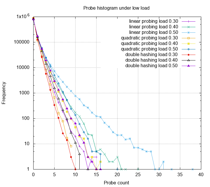
This is a histogram of probe counts. The Y axis is log scale. One can see that other than linear probing, most probes are below 15. Double hashing gives us smallest probe counts, however each of the probe has high probability trigger a cpu cache miss, therefore is slower in practice. Next, we look at these methods under high load.
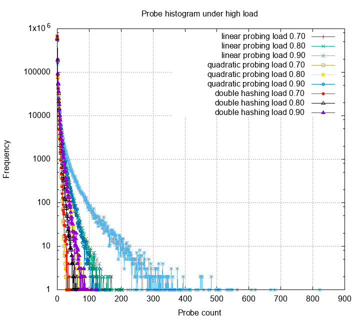
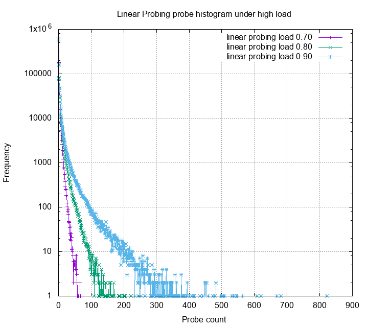
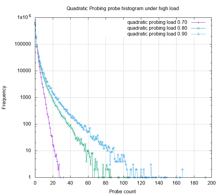
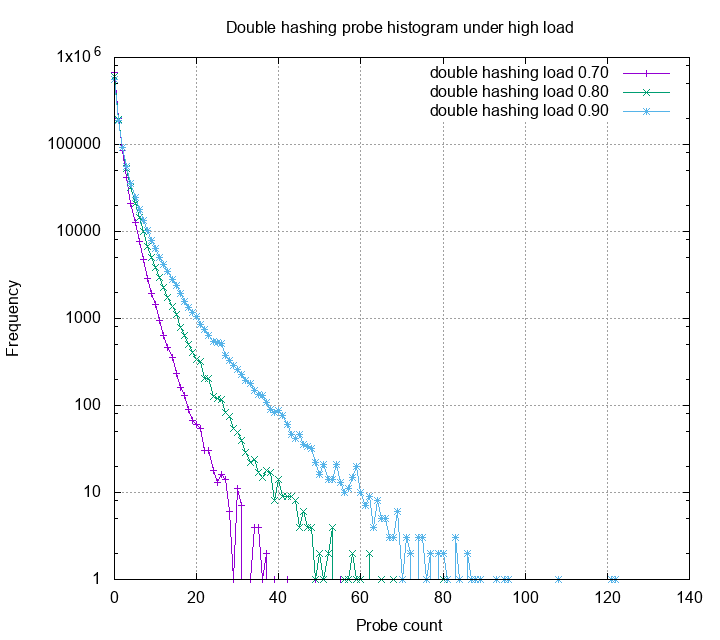
The probe distribution now have a very high variance. Obviously, many probes exceeds the 20 threshold, some even reach 800. Linear probing, among the other methods, has very bad variance under high load. Quadratic probing is slightly better, but still have some probes higher than 100. Double hashing still gives the best probe statistics. Below is the zoom in for each probe strategies:
Robin Hood Hashing for the rescue
The robin hood hashing heuristic is simple and clever. When a collision occur, compare the two items’ probing count, the one with larger probing number stays and the other continue to probe. Repeat until the probing item finds an empty spot. For more detailed analysis checkout the original paper. Using this heuristic, we can reduce the variance dramatically.
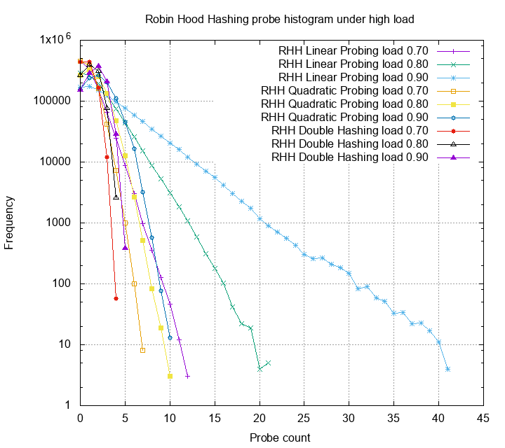
The linear probing now have the worst case not larger than 50, quadratic probing has the worst case not larger than 10, and double hashing has the worst case not larger than 5! Although robin hood hashing adds some extra cost on insert and deletion, but if your table is read heavy, it’s really suitable for the job.
Dive deep and ask why
From engineering perspective, the statistics are sufficient to make design decisions and move on to next steps (though, hopscotch and cuckoo hashing was not tested). That what I did 3 months ago. However, I could never stop asking why. How to explain the differences? Can we model the distribution mathematically?
The analysis on linear probing can trace back to 1963 by Donald Knuth. (It was an unpublished memo dated July 22, 1963. With annotation “My first analysis of an algorithm, originally done during Summer 1962 in Madison”). Later on the paper worth to read are:
- Svante Janson, 2003, INDIVIDUAL DISPLACEMENTS FOR LINEAR PROBING HASHING WITH DIFFERENT INSERTION POLICIES
- Alfredo Viola, 2005, Distributional analysis of Robin Hood linear probing hashing with buckets
- Alfredo Viola, 2010, Distributional Analysis of the Parking Problem and Robin Hood Linear Probing Hashing with Buckets
Unfortunately, these research are super hard. Just linear probing (and its robin hood variant) is very challenging. Due to my poor survey ability, I yet to find a good reference to explain what causes linear probing, quadratic probing and double hashing differ on the probe distribution. Though building a full distribution model is hard, but creating a simpler one to convince myself turns out is not too hard.
Rich get richer
The main reason why linear probing (and probably quadratic probing) gets high probe counts is rich get richer: if you have a big chunk of elements, they are more likely to get hit; when they get hit, the size of the chunk grows, and it just get worse.
Let’s look at a simplified case. Say the hash table only have 5 items, and all the items are in one consecutive block. What is the expected probing number for the next inserted item?
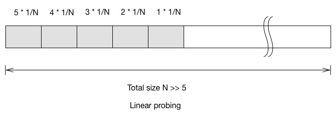
See the linear probing example above. If the element get inserted to bucket 1, it has to probe for 5 times to reach the first empty bucket. (Here we start the probe sequence from index 0; probe number = 0 means you inserted to an empty spot without collision). The expectation probing number for next inserted item is
For quadratic probing, you’ll have to look at each of the item and track where it first probe outside of the block.
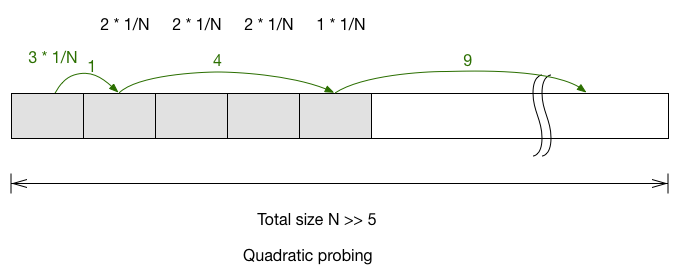
The expected probe number for next item in quadratic probing is $\frac{3+2+2+2+1}{N} = \frac{10}{N}$. Double hashing is the easiest: $1\cdot\frac{5}{N}+2\cdot(\frac{5}{N})^2+3\cdot(\frac{5}{N})^3+\cdots$ If we only look at the first order (because N » 5), then we can simplify it to $\frac{5}{N}$.
- Linear probing: $\frac{15}{N}$
- Quadratic probing: $\frac{10}{N}$
- Double hashing: $\sum_{i=1} i\cdot(\frac{5}{N})^i$
The expected probe number of next item shows that linear probing is worse than other method, but not by too far. Next, let’s look at what is the probability for the block to grow.
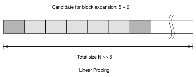
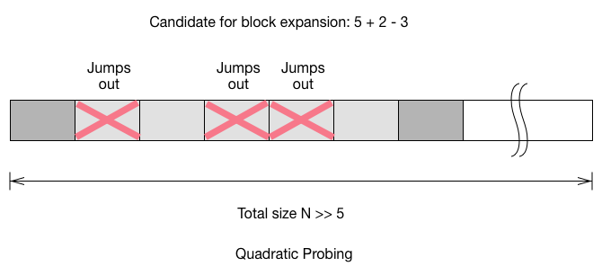
To calculate the probability of the block to grow on next insert, we have to account the two buckets which connected to the block. For linear probing, the probability is $\frac{5+2}{N}$. For quadratic probing, we add the connected block, but we also have to remove the buckets which would jump out during the probe. For double hashing, the probability to grow the block has little to do with the size of the block, because you only need to care the case where it inserted to the 2 connected buckets.
- Linear probing: $\frac{7}{N}$
- Quadratic probing: $\frac{4}{N}$
- Double hashing: $\frac{2}{N}\cdot\sum_{i=0}(\frac{5}{N})^i = \frac{2}{N}\cdot\frac{N}{N-5} = \frac{2}{N-5}$
Using the same calculation, but making the block size as a variable, we can now visualize the block growth of linear probing, quadratic probing, and double hashing.
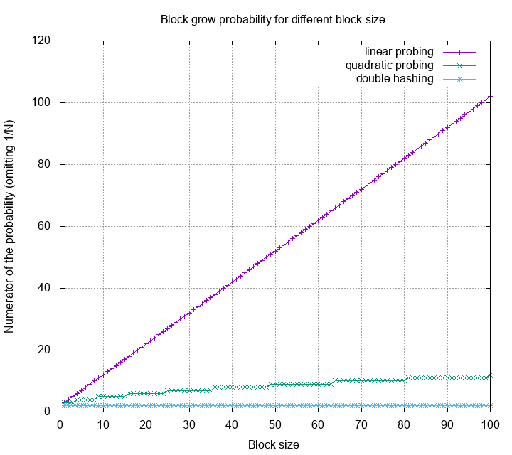
This is not a very formal analysis. However, it gives us a sense of why the rate of linear probing getting worse is way larger than the others. Not only knowing which one is better than the other, but also knowing how much their differences are.
How about the robin hood variant of these three probing methods? Unfortunately, I wasn’t able to build a good model that can explain the differences. A formal analysis on robin hood hashing using linear probing were developed by Viola. I yet to find a good analysis for applying robin hood on other probing method. If you find it, please leave a comment!
Conclusion
Writing a (chaining) hash table to pass an interview is trivial, but writing a good one turns out to be very hard. The key for writing high performance software, is stop guessing.
Measure, measure, and measure. Program elapsed time is just one of the sample point, and can be biased by many things. To understand the program runtime performance, we need to further look at program internal statistics (like probe distribution in this article), cpu cache misses, memory usage, page fault count, etc. Capture the information, and analyze it scientifically. This is the only way to push the program to its limit.
This my first article of “Learn hash table the hard way” series. In the following post I’ll present more angles on examining hash table performance. Hope you enjoy it!