<![CDATA[Carpe diem (Felix's blog)]]>2017-08-06T21:30:21-07:00http://www.idryman.org/Octopress<![CDATA[learn hash table the hard way -- part 3: probe distributions and run time performance]]>2017-08-06T09:03:00-07:00http://www.idryman.org/blog/2017/08/06/learn-hash-table-the-hard-way-3In last two post I gathered the probe statistics in various scenarios.
How does it impact the actual performance? I wrote some benchmarks this
weekend and got useful results.
We know that hash table has O(1) amortized random read. It’s easy
to tell the overall throughput in regular benchmarks. Nevertheless,
it’s harder to know the performance of the worst cases: some keys
has much longer probes than others. Does the performance degrade
by a lot, or not so much? This is critical for applications that
requires real time processing on key value look up.
In order to find the keys with potential high latency,
I designed the experiments as follows:
Insert all keys into the hash table and key buffers.
Sort the keys in the key buffer by its probe count in the hash
table.
Test the table random read throughput from different key range in
the key buffer, where the later key range should have the larger
probe count.
My assumption is, the key look up performance should highly relate to
the key probing count. In my
first post of the learn hash table the hard way, I showed
that robin hood hashing can reduce the probe count variance
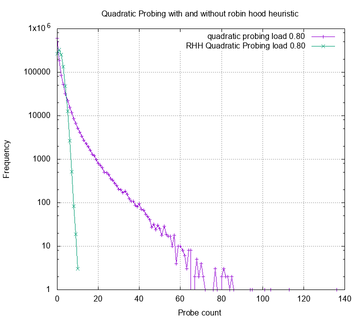
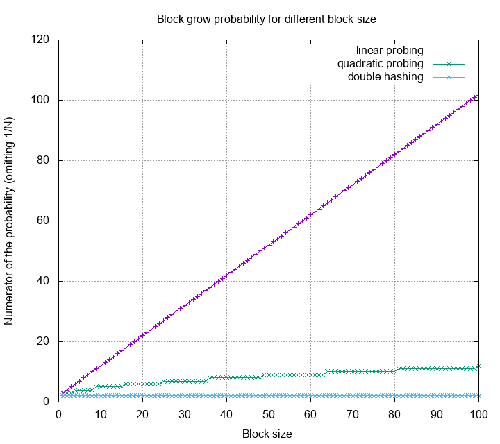
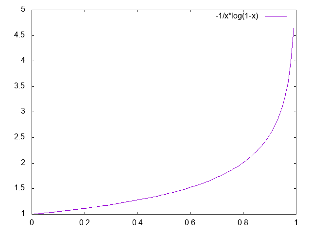
significantly. The plot below compares quadratic probing under 80%
load and quadratic robin hood hashing under 80% load:
Actually, the mean of quadratic probing is slightly better than quadratic
robin hood hashing (1.3 vs 1.45). However the probe count variance of
quadratic probing is visibly way larger than its robin hood siblings.
We’d expect the performance reflects such difference.
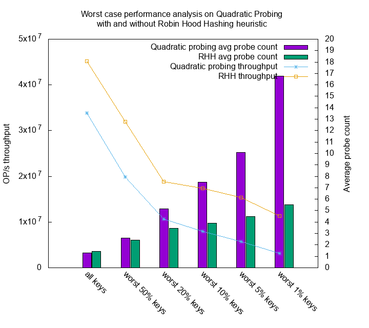
It actually does. The average read throughput of quadratic probing
over all keys is 33,822,611 op/s, but for the worst 1% keys it only has
throughput of 3,137,599 op/s. The difference is 10x. On the other hand,
the throughput of all keys in robin hood hashing is 45,167,612 op/s, and
the throughput of its worst 1% keys is 11,275,010. The difference is 4x.
There’s another interesting observation. Although quadratic probing
has smaller mean of probes compare to robin hood hashing, it’s total
throughput doesn’t win. My guess is having too many large probes would
cause bad cache efficiency.
For instance, all probes in robin hood hashing are within 10 probes.
In this experiments I use 6 bytes for key, 1 byte for key existence
marker, and 8 bytes for value. 10 probes roughly converts to 100 buckets,
each of size 6 + 1 + 8 = 15 bytes. Thus the worst case it need to
walk through 1500 bytes, but only very few items need to go that far.
On the other hand, there’s at least 100 items having probes larger than
40 probes, which takes 24000 bytes. For such a long distance you’ll
have lots of CPU cache misses. This is my best guess of why robin
hood hashing overtakes quadratic probing even when the average
probe count is slightly larger.
I haven’t find much discussion on hash table performance corresponding
to probe distribution. My hypothesis and experiments are in early
stages. If you find any similar experiments, research, or report,
please leave a comment! I’d like to reach out and learn more.
]]><![CDATA[learn hash table the hard way -- part 2: probe distributions with deletions]]>2017-07-18T19:02:00-07:00http://www.idryman.org/blog/2017/07/18/learn-hash-table-the-hard-way-2In the last post I demonstrated probe distributions under six insertion
schemes: linear probing, quadratic probing, double hashing, and their
robin hood hashing variants. Knowing the probe distribution of insertion
is useful for static hash tables, but does not model the hash table with
frequent updates. Therefore I made some experiments for such scenario,
and found the results are very interesting.
Same disclaimer. I now work at google, and this project
(OPIC including the hash table implementation) is approved by google
Invention Assignment Review Committee as my personal
project. The work is done only in my spare time on my own machine,
and does not use and/or reference any of the google internal resources.
Deletion in open addressing schemes
In most open addressing schemes, deletion is done by marking the
bucket with a tombstone flag. During the next insertion, both
empty bucket and tombstone bucket can hold new items. During
look ups, seeing an empty bucket means the key was not found, but if
you saw a tombstone bucket you must continue probing. If too many
items got deleted and causes the load smaller than a threshold,
shrink the hash table and re-insert the non-tombstone items.
Table with high insertion/deletion rate
Consider the following: you are maintaining a large key value store
which uses hash table internally. The key value store has many
keys inserted and deleted frequently, but the total keys remains the
same (limited by capacity or ttl). Let’s assume all keys have equal
probability to get deleted. The keys with low probing count would
eventually get deleted at sometime, while the newly inserted key
may occur with high probing count because the table is always
under high load. An interesting question rises:
Will the probe number continue growing?
Or the probe number converges to certain distribution?
I yet to see mathematical analysis on this problem. If you know a good
reference, please leave a comment. Finding the formal bound were too
hard for me, so I designed a small experiment to understand the
effect. The experiment will have ten rounds. In the first round,
insert 1M items. In the next nine rounds, delete an item and insert a
new item for 1M times. I only tested this experiment on quadratic
probing scheme and robin hood with quadratic probing.
Quadratic probing with deletion
Quadratic probing is used in dense hash map. This is one of the
fastest hash table with wide adoption, therefore worth the study.
For this experiment I didn’t use dense hash map, instead I wrote
a small C program with same probing algorithm and record the probe counts.
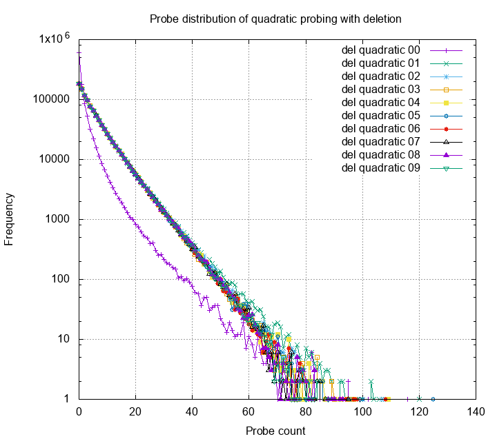
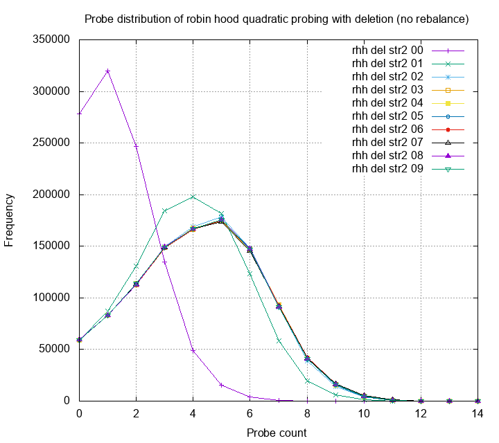
The chart below is a histogram of probe count for quadratic probing.
Each line is the distribution of probes of different rounds; 00 is
insertion only round, and others have pair of deletion and insert.
Each round have 1M items inserted and/or deleted. The table is under
80% load.
Surprisingly, the probe histogram converges to a shape after
one round. This means that the hash table performance will
drop after one round of replacing all the elements, but will reach
to a steady state and stop getting worse. The shape of the steady
distribution looks like a exponential distribution. I wonder can
we use this property and further derive other interesting properties?
Robin hood hash with deletion
In the robin hood hashing thesis the author conjectured
that having deletion would cause the mean of probe count increase
without bound, but the variance would remain bounded by small constant.
Paul Khuong and Emmanuel Goossaert pioneered
to approach this problem. The intuition is fill the deleted bucket
by scanning forward candidate buckets. See Emmanuel’s post
for more detail.
Inspired by their robin hood linear probing deletion, I created one
for robin hood quadratic probing. The idea is similar, except the
candidates are not limited to its neighbors. I have to scan through
possible candidates from largest probe number, and check is the
candidate valid to fill the spot. There are some other tricks I did
to make sure the iteration done in deletion is bounded, but isn’t
important in this post.
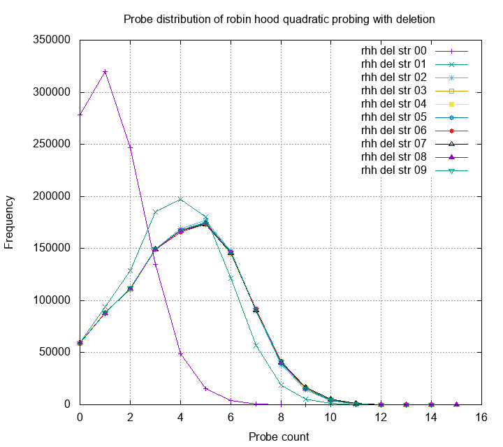
The probe distribution using this idea is shown as follows:
The result is also very good. Both the mean and variance is smaller
than naive quadratic probing. Luckily, the conjecture of unbounded
mean wasn’t true, it converges to a certain value! Recall from last
post; we want to know what is the worst case probe (< 20 for 1M inserts)
and the average case. Even with lots of inserts and deletes, the
mean is still in constant bound, and the worst case is not larger than
O(log(N)).
How about robin hood hashing without the re-balancing strategy? Again,
the results blows my mind:
It’s actually very identical to my carefully designed deletion method.
When I first see the experiment result, I was quite shocked. I can do
nothing but to accept the experiment result, and adapt new
implementation. In my journey of optimizing hash tables, I found
clever ideas often failed (but not always!). Finding a good
combination of naive and clever ideas for good performance is tough. I
did it by doing exhaustive search of different combinations, then
carefully measure and compare.
In OPIC robin hood hashing I initially only interested at
building static hash table with high load. However, after this
experiments I concluded that robin hood hashing has good potential for
dynamic hash table as well.
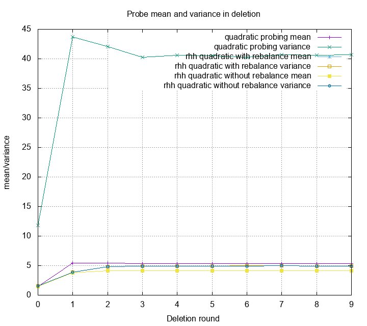
Aggregated stats
Last but not least, let’s look at mean and variance for each method
and each round.
The mean of quadratic probing and robin hood quadratic probing actually
doesn’t differ by much. Only a little bit after first round. The difference
of variance is huge because that’s what robin hood hashing is designed for.
Summary
In the first two post of learn hash table series, we examined probe
distributions of various methods and scenarios. In the next post I’ll
show how these distribution reflects on actual performance. After all,
these experiments and study were meant to leads to better engineering
result.
]]><![CDATA[learn hash table the hard way -- part 1: probe distributions]]>2017-07-04T13:05:00-07:00http://www.idryman.org/blog/2017/07/04/learn-hash-table-the-hard-wayIn the last 4 months I’ve been working on how to implement a good hash table
for OPIC (Object Persistence in C). During the development, I made
a lot of experiments. Not only for getting better performance, but also knowing
deeper on what’s happening inside the hash table. Many of these findings are
very surprising and inspiring. Since my project is getting mature, I’d get
a pause and start writing a hash table deep dive series. There was a lot of
fun while discovering these properties. Hope you enjoy it as I do.
Same disclaimer. I now work at google, and this project
(OPIC including the hash table implementation) is approved by google
Invention Assignment Review Committee as my personal
project. The work is done only in my spare time on my own machine,
and does not use and/or reference any of the google internal resources.
Background
Hash table is one of the most commonly used data structure. Most standard
library use chaining hash table, but there are more options in
the wild. In contrast to chaining, open addressing does
not create a linked list on bucket with collision, it insert the item
to other bucket instead. By inserting the item to nearby bucket, open
addressing gains better cache locality and is proven to be faster in many
benchmarks. The action of searching through candidate buckets for insertion,
look up, or deletion is known as probing. There are many probing strategies:
linear probing, quadratic probing, double hashing, robin
hood hasing, hopscotch hashing, and cuckoo hashing.
Our first post is to examine and analyze the probe distribution among these
strategies.
To write a good open addressing table, there are several factors to consider:
1. load: load is the number of bucket occupied over the bucket
capacity. The higher the load, the better the memory utilization is.
However, higher load also means the probability to have collision is higher.
2. probe numbers: the number of probes is the number of look up to reach the
desired items. Regardless of cache efficiency, the lower the total probe
count, the better the performance is.
3. CPU cache hit and page fault: we can count both the cache hit and page
fault analytically and from cpu counters. I’ll write such analysis in later
post.
Linear probing, quadratic probing, and double hashing
Linear probing can be represented as a hash function of a key and a
probe number $h(k, i) = (h(k) + i) \mod N$. Similarly, quadratic
probing is usually written as $h(k, i) = (h(k) + i^2) \mod N$. Double
hashing is defined as $h(k, i) = (h1(k) + i \cdot h2(k)) \mod N$.
Quadratic probing is used by dense hash map. In my knowledge
this is the fastest hash map with wide adoption. Dense hash map set
the default maximum load to be 50%. Its table capacity is bounded
to power of 2. Given a table size $2^n$, insert items $2^{n-1} + 1$,
you can trigger a table expansion, and now the load is 25%. We can
claim that if user only insert and query items, the table load is
always within 25% and 50% (the table may need to expand at least once).
I implemented a generic hash table to simulate dense hash
map probing behaviors. Its performance is identical to dense hash
map. The major difference is I allow non power of 2 table size, see
my previous post for why the performance does not degrade.
I setup the test with 1M inserted items. Each test differs in its load
(by adjusting the capacity) and probing strategies.
Although hash table is O(1) on amortized look up, we’ll still hope the
worst case not larger than O(log(N)), which is log(1M) = 20 in this case.
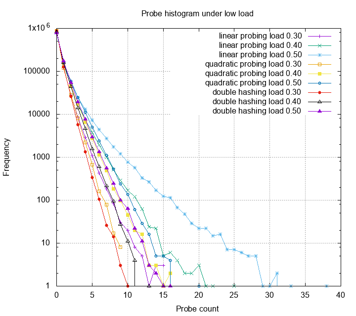
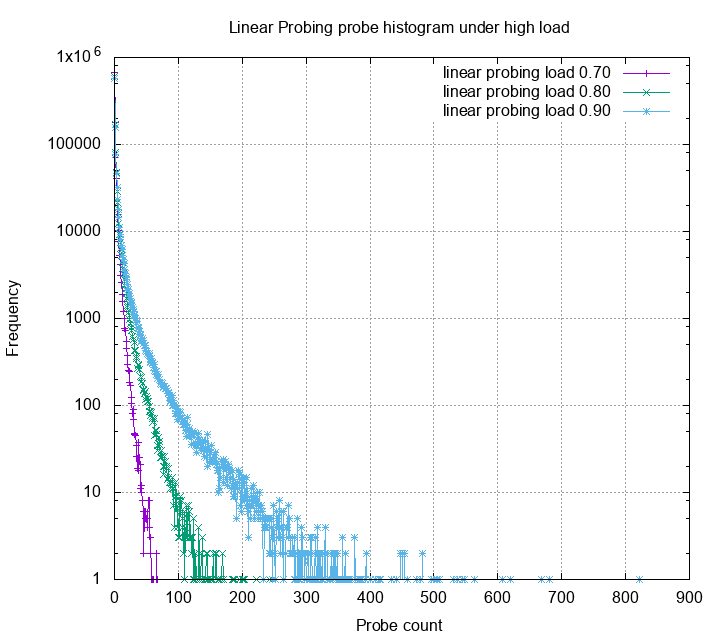
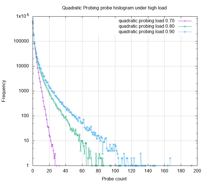
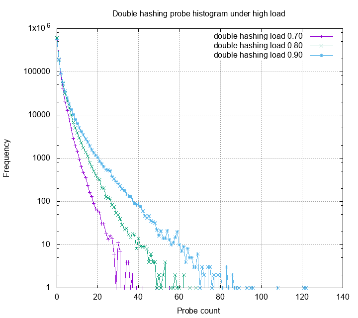
Let’s first look at linear probing, quadratic
probing and double hashing under 30%, 40%, and 50% load.
This is a histogram of probe counts. The Y axis is log scale. One can
see that other than linear probing, most probes are below 15. Double
hashing gives us smallest probe counts, however each of the probe has
high probability trigger a cpu cache miss, therefore is slower in
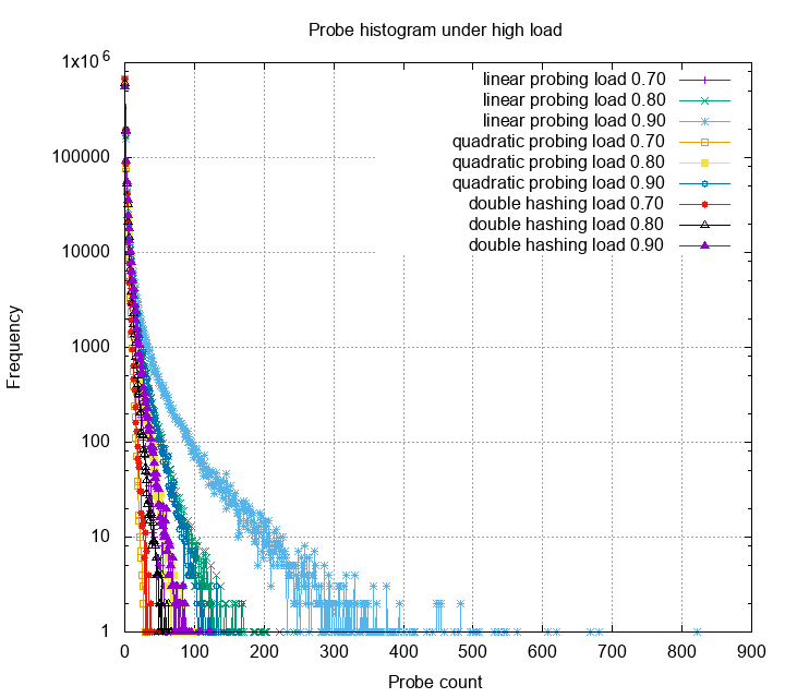
practice. Next, we look at these methods under high load.
The probe distribution now have a very high variance. Obviously, many
probes exceeds the 20 threshold, some even reach 800.
Linear probing, among the other methods, has very bad variance under
high load. Quadratic probing is slightly better, but still have some
probes higher than 100. Double hashing still gives the best probe
statistics. Below is the zoom in for each probe strategies:
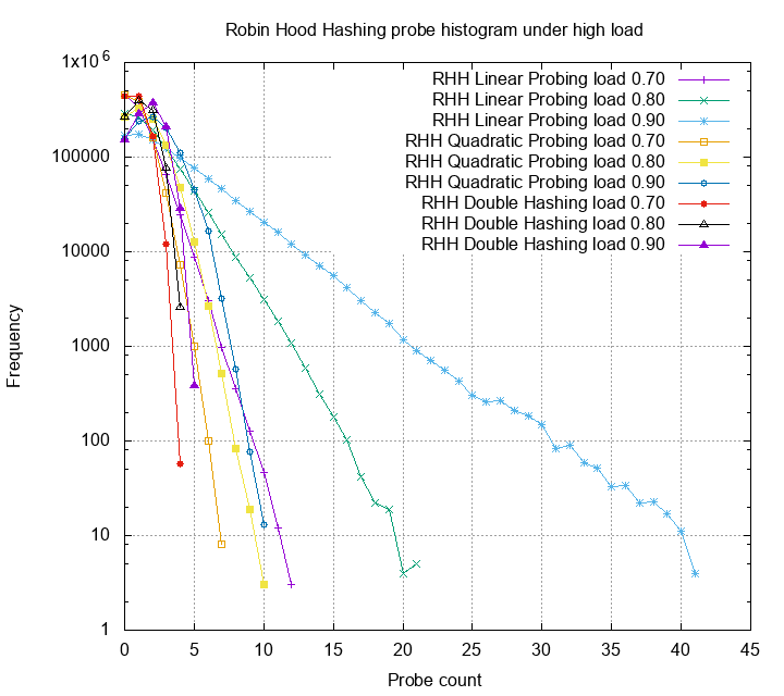
Robin Hood Hashing for the rescue
The robin hood hashing heuristic is simple and clever. When
a collision occur, compare the two items’ probing count, the one
with larger probing number stays and the other continue to probe.
Repeat until the probing item finds an empty spot. For more detailed
analysis checkout the original paper.
Using this heuristic, we can reduce the variance dramatically.
The linear probing now have the worst case not larger than 50,
quadratic probing has the worst case not larger than 10, and
double hashing has the worst case not larger than 5! Although
robin hood hashing adds some extra cost on insert and deletion,
but if your table is read heavy, it’s really suitable for the job.
Dive deep and ask why
From engineering perspective, the statistics are sufficient to make
design decisions and move on to next steps (though, hopscotch and
cuckoo hashing was not tested). That what I did 3 months ago. However,
I could never stop asking why. How to explain the differences? Can
we model the distribution mathematically?
The analysis on linear probing can trace back to 1963 by Donald Knuth.
(It was an unpublished memo dated July 22, 1963. With annotation “My
first analysis of an algorithm, originally done during Summer 1962 in
Madison”). Later on the paper worth to read are:
Unfortunately, these research are super hard. Just linear probing (and its
robin hood variant) is very challenging. Due to my poor survey ability, I
yet to find a good reference to explain what causes linear probing, quadratic
probing and double hashing differ on the probe distribution. Though building
a full distribution model is hard, but creating a simpler one to convince myself
turns out is not too hard.
Rich get richer
The main reason why linear probing (and probably quadratic probing) gets high
probe counts is rich get richer: if you have a big chunk of elements, they
are more likely to get hit; when they get hit, the size of the chunk grows,
and it just get worse.
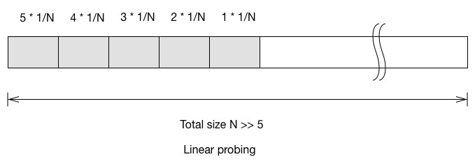
Let’s look at a simplified case. Say the hash table only have 5 items, and all
the items are in one consecutive block. What is the expected probing number for
the next inserted item?
See the linear probing example above. If the element get inserted to bucket 1,
it has to probe for 5 times to reach the first empty bucket. (Here we start the
probe sequence from index 0; probe number = 0 means you inserted to an empty
spot without collision). The expectation probing number for next inserted item
is
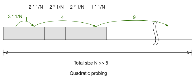
For quadratic probing, you’ll have to look at each of the item and track
where it first probe outside of the block.
The expected probe number for next item in quadratic probing is
$\frac{3+2+2+2+1}{N} = \frac{10}{N}$. Double hashing is the easiest:
$1\cdot\frac{5}{N}+2\cdot(\frac{5}{N})^2+3\cdot(\frac{5}{N})^3+\cdots$
If we only look at the first order (because N » 5), then we can
simplify it to $\frac{5}{N}$.
The expected probe number of next item shows that linear probing is
worse than other method, but not by too far. Next, let’s look at
what is the probability for the block to grow.
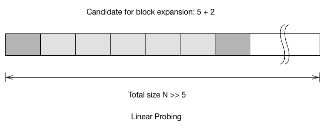
To calculate the probability of the block to grow on next insert, we
have to account the two buckets which connected to the block. For linear
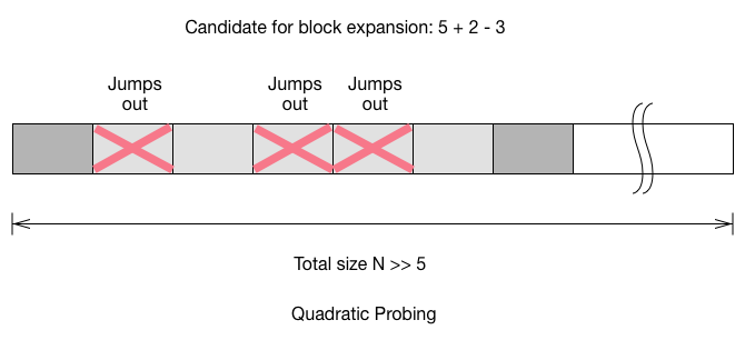
probing, the probability is $\frac{5+2}{N}$. For quadratic probing, we
add the connected block, but we also have to remove the buckets which
would jump out during the probe. For double hashing, the probability
to grow the block has little to do with the size of the block, because
you only need to care the case where it inserted to the 2 connected
buckets.
Using the same calculation, but making the block size as a variable,
we can now visualize the block growth of linear probing, quadratic
probing, and double hashing.
This is not a very formal analysis. However, it gives us a sense of why
the rate of linear probing getting worse is way larger than the others.
Not only knowing which one is better than the other, but also knowing
how much their differences are.
How about the robin hood variant of these three probing methods?
Unfortunately, I wasn’t able to build a good model that can explain
the differences. A formal analysis on robin hood hashing using linear
probing were developed by Viola. I yet to find a good analysis
for applying robin hood on other probing method. If you find it, please
leave a comment!
Conclusion
Writing a (chaining) hash table to pass an interview is trivial, but writing
a good one turns out to be very hard. The key for writing high performance
software, is stop guessing.
Measure, measure, and measure. Program elapsed time is just one of the
sample point, and can be biased by many things. To understand the
program runtime performance, we need to further look at program
internal statistics (like probe distribution in this article), cpu
cache misses, memory usage, page fault count, etc. Capture the
information, and analyze it scientifically. This is the only way to
push the program to its limit.
This my first article of “Learn hash table the hard way” series. In
the following post I’ll present more angles on examining hash table performance.
Hope you enjoy it!
]]><![CDATA[Writing a memory allocator for fast serialization]]>2017-06-28T12:19:00-07:00http://www.idryman.org/blog/2017/06/28/opic-a-memory-allocator-for-fast-serializationIn my last post, I briefly introduced OPIC (Object Persistance
in C), which is a general serialization framework that can
serialize any object without knowing its internal layout.
In this post, I’ll give a deeper dive on how it works.
Still with the same disclaimer. I now work at google, and this project
(OPIC including the hash table implementation) is approved by google
Invention Assignment Review Committee as my personal
project. The work is done only in my spare time on my own machine,
and does not use and/or reference any of the google internal resources.
Rationale: key-value store performance
Key-value data retrieval is probably the most commonly used abstraction
in computer engineering. It has many forms: NoSQL key value store, embedded
key value store, and in-memory data structures. In terms of algorithm
complexity, they are all having O(1) amortized insertion, deletion, and
query time complecity. However, the actual performance ranges from 2K QPS
(query per second) up to 200M QPS.
To make it easier to reason about, here I only compare read only performance.
Furthermore, it’s single node, single core. In this setup, the data store
should not have transaction or WAL (write ahead log) overhead; if table locking
was required, only the reader lock is needed; if the data was stored on disk,
the read only load should trigger the data store to cache it in memory, and
the overall amortized performance theoratically should be close to what
in-memory data structure can achieve.
The first tier of data stores we look at, are the full featured SQL/NoSQL
database which support replication over cluster of nodes. A report created
by engineers at University of Toronto is a good start:
Solving Big Data Challenges for Enterprise Application Performance
Management. In this report they compared Cassandra,
Voldemort, Redis, HBase, VoltDB, and MySQL. Unfortunately, their report
doesn’t have 100% read only performance comparison, only 95% read is
reported.
Cassandra: 25K QPS
Voldemort: 12K QPS
Redis: 50K QPS
HBase: 2.5K QPS
VoltDB: 40K QPS
MySQL: 25K QPS
Some report gives even worse performance numbers. In
this nosql benchmark, 100% read, Cassandra, HBase, and mongo
are all having throughput lower than 2K QPS.
The performance of the databases above may be biased by network,
database driver overhead, or other internal complexities. We now look
at the second tier, embedded databases: LMDB, LevelDB, RocksDB,
HyperLevelDB, KyotoCabinet, MDBM and BerkelyDB all falls into this
category. The comparison of first four databases can be found in
this influxdb report.
100M values (integer key)
LevelDB: 578K QPS
RocksDB: 609K QPS
HyperLevelDB: 120K QPS
LMDB: 308K QPS
50M values (integer key)
LevelDB: 4.12M QPS
RocksDB: 3.68M QPS
HyperLevelDB: 2.08M QPS
LMDB: 5.89M QPS
The performance report from MDBM benchmark is also interesting. They
only provide the latency number though.
MDBM: 0.45 us, ~= 2M QPS (?)
LevelDB: 5.3 us, ~= 0.18 QPS (?)
KyotoCabinat: 4.9 us, ~= 0.20 QPS (?)
BerkeleyDB: 8.4 US, ~= 0.12 QPS (?)
I’m guessing the performance number can be very different when the
keys are different. In this LMDB benchmark, LevelDB
only achieves 0.13M QPS. We can see huge difference in the following
in memory hash tables. I ran these benchmarks myself. The code is hosted
at hash_bench.
key: std::string
std::unordered_map: 5.3M QPS
sparse_hash_map: 4.4M QPS
dense_hash_map: 9.0M QPS
key: int64
std::unordered_map: 106M QPS
dense_hash_map: 220M QPS
This is the state of the art I have surveyed and experimented so far.
Clearly, the in memory data structure out performs all the other solutions.
There’s a big gap between the data store that can save to disk, versus
pure in-memory solutions. Can we fill the gap, and create a data store
with competitive performance to the best hash tables? This motivates me
to build OPIC (object persistence in C), where developer can focus on
writing fast in-memory data structures, and offload the serialization to
a general framework.
Rethink serialization
I like the clear definition in wikipedia that describes serialization:
serialization is the process of translating data structures or
object state into a format that can be stored (for example, in a
file or memory buffer) or transmitted (for example, across a network
connection link) and reconstructed later (possibly in a different
computer environment).
In our case, we want to minimize this translation cost. The smaller
the translation cost, the faster the system can load the data.
Pushing this idea to extreme, what if the object have the same
representation in memory and on disk? This concept is not new.
Many modern serialization framework treats the serialized object
as an actual in memory object with accessors. Protobuf
and thrift are two implementation for such idea. However,
neither protobuf nor thrift is capable to represent general
data structures like linked list, trees, or (large) hash tables. These
solutions lack of pointers; the only supported object relationship is
inline object or inline list of objects.
Why is pointer hard for serialization? If you simply copy the pointer
value for serialization, the address it pointed at would not be valid
after you restore it from disk. Most general serialization framework
would have to walk though all the related object user attempt to
serialize, copy all the objects, either inline the object or create
a special mapping of objects for cross references. In the current
state of the art, either you drop the support of pointer and get
minimized translation cost, or you pay high translation fee (walk
through objects) for general data structure serialization. How
can we do better?
Turns out, once you have a good way to represent the pointer value,
you gain the benefits of both solution: cheap serialization cost
and freedom to implement all types of data structures.
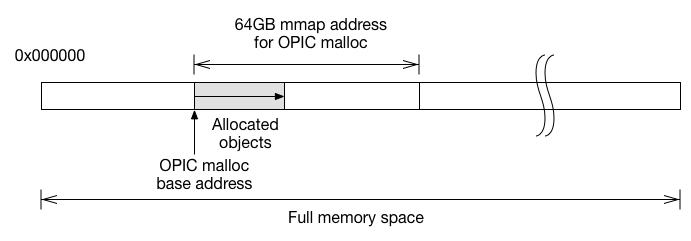
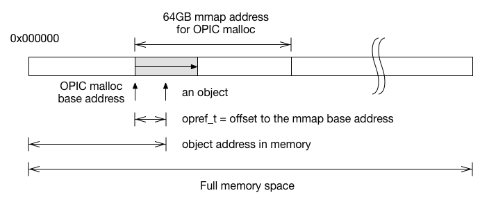
Key idea: Put a bound on pointer addresses
Pointers are hard to serialize because it can point to anywhere
in the full virtual memory space. The solution is pretty straight
forward, simply bound the objects into a heap space we control.
Having all objects bounded in one memory space, serialization is
simply dumping the shaded memory out, and de-serialization is mmap the
file back in memory. What if the objects contain pointers? Instead of
using pointers, we use the offset to the mmap base address to
reference objects. When accessing objects, we add the base address
back to the offset to reconstruct the pointer. Since we only use
the offset opref_t to store the pointer, even if the whole mmap
got mapped to a different address, we can still access the object
by adding a different base address to the offset. If we can ensure
all the pointers within the block are stored as opref_t, the whole
block of memory can be dumped out without any translation!
Implementation challenges
Having zero translation (serialization/de-serialization) cost is very
attractive. However, building a POC took me a year (actually this is
the third version, but I omitted the details). Here are the challenges
I’ve found during the development.
All objects need to be bounded in a memory chunk. Therefore I have
to write a full featured memory allocator. Writing a good one is very
time consuming.
Programming languages with run-time pointers, like vtables, pointers
in existing containers, etc. cannot be used in this framework. All
containers (hash tables, balanced tress) need to be rebuilt from ground up.
C++, Rust, Go all have their run-time pointers and cannot be used. The only
language I can use is pure C. (This is why the project is named Object
Persistence in C).
Serialized object cannot be transferred between architectures like
32bit/64bit, little endian or big endian. Depends on the use case, this
problem might be minor.
These constraints shapes OPIC. The core OPIC API is a memory manager
for allocating C objects. All the objects created by OPIC would be
bounded in the 64GB mmap space. The 64GB size were chosen to hold
enough objects, while user can load many OPIC mmap files in the same
process.
Using OPIC malloc is very identical to standard malloc, except user
need to specify an OPHeap object where the object would allocated in.
1234567
OPHeap*heap;// Initialize a 64GB OPIC heap via mmapOPHeapNew(&heap);// pointer for accessing the objectint*a_ptr=OPMalloc(heap,sizeof(int));// deallocate an object does not require specifying the heapOPDealloc(a_ptr);
What makes it different to regular malloc is, user can write the whole
heap to disk and restoring back via file handles.
To make your data structure work, you must store your pointer as
opref_t instead of regular pointer. Converting a pointer to opref_t
and vise versa is similar, except when restoring opref_t back to
pointer user must specify which OPHeap its belongs to.
123456
// Convert the pointer to a offset to the OPHeap base address// The pointer must be a pointer created by OPHeapopref_ta_ref=OPPtr2Ref(a_ptr);// Add the offset a_ref with OPHeap base address to restore// the pointer.int*a_ptr=OPRef2Ptr(heap,a_ref);
In regular programs, user keeps their own reference of the allocated
objects. However, in the OPIC case, user would lost track of the
objects they allocated after the heap is serialized. This problem
can be solved by saving the pointers to the root pointer slot
that OPIC provides. Each OPIC heap offers 8 root pointer slot.
12345678910111213141516171819
/** * @relates OPHeap * @brief Store a pointer to a root pointer slot in OPHeap. * * @param heap OPHeap instance. * @param ptr the pointer we want to store in root pointer slot. * @param pos index in the root pointer slot. 0 <= pos < 8. */voidOPHeapStorePtr(OPHeap*heap,void*ptr,intpos);/** * @relates OPHeap * @brief Restore a pointer from specified root pointer slot. * * @param heap OPHeap instance. * @param pos index in the root pointer slot. 0 <= pos < 8. * @return The pointer we stored in the root pointer slot. */void*OPHeapRestorePtr(OPHeap*heap,intpos);
This API has been through many iterations. In the early version
it was a bunch of C macros for building serializable objects.
Fortunately it’s simplified and became more powerful and general
to build serializable applications. I believe it is now simple
enough and only require a little C/C++ programming skill to master.
Check out the OPIC Malloc API
for details
Performance
OPIC can be used for general data serialization. The first data structure
I implemented is Robin Hood hash table – a hash map variant which has
good memory utilization without performance degradation. Memory utilization
affects how large the serialized file is, therefore is a one of the main
focus for writing OPIC containers. The details for keeping the memory footprint
small is in my previous post.
The performance ends up super good: 9M QPS for in memory hash table.
For non-cached performance, I tested it by de-serializing on every
query. Every query would have to load the whole file back in memory
via mmap, then page fault to load the query entry. For this test I
got 2K QPS, which is 0.0005 second latency per load. Both cached
and non-cached performance are very promising, and perhaps is very
close to the upper bound for such application could perform.
Current and future scope of OPIC
Currently OPIC is implemented for building static data structures.
Build the data structure once, then make it immutable. User can
preprocess some data and store it with OPIC for later use. This
is the minimal viable use case I can think of for the initial release,
but OPIC can do more.
First of all, I want to make OPIC easier to access for more programmers.
Building high level application in pure C is time consuming, therefore
I’ll be writing language wrappers for C++, Python, R, and Java so that
more people can benefits the high speed serialization.
Second, I’ll make OPIC able to mutate after first serialization. High
level language user may treat OPIC as database of data structures
that one can compose. This kind of abstraction is different to
traditional database where program logic have to map to set of
records. I believe this will bring in more creative usage of new
types of applications.
Finally, I’d want to make OPIC to work on distributed applications.
I used to work on Hadoop and big data applications. I always wonder,
why people rarely talks about complexity and data structures in big
data world? Why there is no framework provide data structure abstraction
for big data? Isn’t the large the data size is, the more important
the complexity and data structure is? Building data structure for
super scale application, is the ultimate goal of OPIC.
Thank you for reading such a long post. If you also feel excited on
what OPIC might achieve, please post your comment. If you want to
contribute, that’s even better! The project page is at
github. Feel free to fork and extend.
Edit (7/15/2017)
After posted on hacker news, some people pointed out that
boost::interprocess
provides similar functionality and approaches.
To make a memory chunck work in different process, they also use special pointer
which are offsets to base address of the mmap. The challenges are identical too.
Any pointer that is unique to the process, like static members,
virtual functions, references, function pointers etc. are forbidden.
All the containers need to be reimplemented like I did.
To make the project succeed, I think the most important part is to provide
good abstractions for users. State of the art containers, simple API to use,
create extensions for other languages to use etc. Now OPIC robin hood hash
container has reached (or beyond) state of the art, I’ll be continue to create
more useful abstractions for people to create persistent objects.
The next container I’ll be working on is compressed trie. This would be a
counter part of hash table. Hash table provides super fast random access,
but there’s a high lower bound on memory usage (though I’m very close to
the limit). For trie, I’ll be focus on make the memory usage as small as
possible. If possible, make it succinct. Hash table can be used as short
term data random look up, while trie can be used to store long term data,
with compression and keeps the ability to do random look up.
]]><![CDATA[Writing a damn fast hash table with tiny memory footprints]]>2017-05-03T18:26:00-07:00http://www.idryman.org/blog/2017/05/03/writing-a-damn-fast-hash-table-with-tiny-memory-footprintsHash table is probably the most commonly used data structure in
software industry. Most implementations focus on its speed instead
of memory usage, yet small memory footprint has significant impact
on large in-memory tables and database hash indexes.
In this post, I”ll provide a step by step guide for writing a modern
hash table that optimize for both speed and memory efficiency. I’ll
also give some mathematical bounds on how well the hash table could
achieve, and shows how close we are to the optimal.
Let me start with a disclaimer. I now work at google, and this project
(OPIC including the hash table implementation) is approved by google
Invention Assignment Review Committee as my personal
project. The work is done only in my spare time with my own machine
and does not use and/or reference any of the google internal resources.
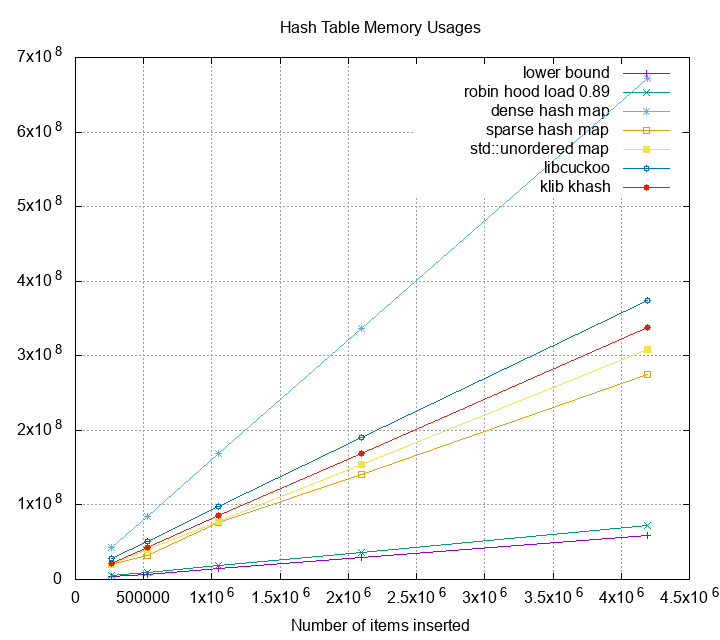
Common hash table memory usages
As mentioned earlier, most hash hash table focus on its speed, not
memory usage. Consequently there’s not much benchmark compares the
memory these hash table implementation consumes. Here is a very basic
table for some high performance hash table I found. The input is 8 M
key-value pairs; size of each key is 6 bytes and size of each value is
8 bytes. The lower bound memory usage is $(6+8)\cdot 2^{23} =$ 117MB
. Memory overhead is computed as memory usage divided by the
theoretical lower bound. Currently I only collect 5 hash table
implementations. More to be added in future.
Memory Usage
Memory Overhead
Insertion Time
Query Time
std::unordered_map
588M
5.03x
2.626 sec
2.134 sec
sparse_hash_map
494M
4.22x
7.393 sec
2.112 sec
dense_hash_map
1280M
10.94x
1.455 sec
1.436 sec
libcuckoo
708M
6.05x
2.026 sec
2.120 sec
klib khash
642M
5.48x
4.232 sec
1.647 sec
The metrics above actually surprises me. For example,
[sparse hash map][shm] is advertised to use 4-10 bits per entry,
but the overhead is actually 4 times the lower bound. If the
hash table were implemented as large key-value store index, and
you have 1 TB of data, you’ll need at least 4-5TB of space to
hold the data. That’s not very space efficient. Can we do better?
Overview of hash table types
There’s two major types of hash table, one is chaining and
the other is open addressing. Chaining is quite common
in most standard libraries, where the collision is handled by
appending items into a linked list headed by the bucket the key is
mapped to. Open addressing uses a different mechanism to handle
collision: the key (and value) is inserted to another bucket if the
bucket it attempt to insert is already occupied.
Open addressing has some clear advantages over chaining. First, it
does not require extra memory allocation. This reduces memory allocation
overhead and can possibly improve cpu caching. Moreover, in open
addressing the developer has more control on memory layout – placing
elements in buckets with certain order to make probing (search on
alternative location for key) fast. Best of all, open addressing
gives us better memory lower bound over chaining.
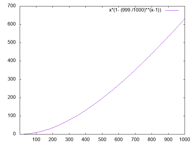
The hash collision rate affects the chaining memory usage. Given a
hash table with $N$ buckets, we insert $M$ elements into the
table. The expected collision number in the table is $M(1 - (1 -
1/N)^{M-1})$. For a table with 1000 buckets the expected collisions
under high loads ($M/N > 80%$) are:
80% -> 440
90% -> 534
100% -> 632
Accounting the extra payload that chaining requires, we can now compute
the lower bound for the overhead under different loads.
load
Chaining
Open Addressing
100%
1.31x
1.00x
90%
1.37x
1.11x
80%
1.47x
1.25x
70%
1.60x
1.42x
50%
2.09x
2.00x
25%
4.03x
4.00x
Here I assume if the collision rate were 60%, half of it is chained
and half of it fits the buckets. The actual number may have some
digits off, but it doesn’t change my conclusion on choosing open
addressing for hash table implementation.
Probing methods
In open addressing, hash collisions are resolved by probing, a search
through alternative buckets until the target record is found, or some
failure criteria is met. The following all belongs to some kinds of
probing strategies:
Linear Probing
Quadratic Probing
Double Hashing
Hopscotch Hashing
Robin Hood Hashing
Cuckoo Hashing
For each of the probing method, we’re interested in their worst case
and average case probing numbers, and is their space bound.
Linear Probing and Quadratic Probing
Linear probing can be represented as a hash function of a key and a
probe number $h(k, i) = (h(k) + i) \mod N$. Similarly, quadratic
probing is usually written as $h(k, i) = (h(k) + i^2) \mod N$. Both
methods has worst case probing count $O(N)$, and are bounded on
space usage. In other words, there no condition where we need to
increase the bucket count and rehash.
Double hashing
Double hashing can be written as
$h(k, i) = (h1(k) + i \cdot h2(k)) \mod N$.
Same as linear probing and quadratic probing, it has worst
case probing count $O(N)$, and is bounded on space usage.
Hopscotch Hashing
Here is the algorithm copied from wikipedia.
This is how the collision is handled
If the empty entry’s index j is within H-1 of entry i, place x
there and return. Otherwise, find an item y whose hash value lies
between i and j, but within H-1 of j. Displacing y to j creates a
new empty slot closer to i. If no such item y exists, or if the
bucket i already contains H items, resize and rehash the table.
This mechanism has a good worst case probing number $O(H)$. However,
since it could resize the hash table, the hash table size is unbounded.
Robin Hood Hashing
The concept for robin hood hashing is simple and clever. When
a collision occur, compare the two items’ probing count, the one
with larger probing number stays and the other continue to probe.
Repeat until the probing item finds an empty spot. For more detailed
analysis checkout the original paper. It’s worth to read.
The expected probing length is
Even under a high load, we still get very good probing numbers.
The best thing about robin hood hashing is it does not expand
the hash table, which is important because we want to build a
hash table with bounded size. This is the probing strategy I chose.
Cuckoo hashing
The following description is also copied from wikipedia.
It uses two or more hash functions, which means any key/value pair
could be in two or more locations. For lookup, the first hash
function is used; if the key/value is not found, then the second hash
function is used, and so on. If a collision happens during insertion,
then the key is re-hashed with the second hash function to map it to
another bucket.
The expected probing number is below 2. However, the load factor has
to be below 50% to achieve good performance. For using 3 hash functions,
the load can increase to 91%. Combining linear/quadratic probing with
cuckoo, the load factor can go beyond 80%. (All numbers comes from
wikipedia).
Optimizing Division for Hash Table Size
I implemented a robin hood hashing prototype a month ago. The prototype
satisfy the low memory footprint, but hard to get it fast. The major
reason is the modulo operation is very slow on most platforms. For example,
on Intel Haswell the div instruction on 64bit integer can take 32-96
cycles. Almost all major hash implementation use power of 2 table size,
so that the modulo is just one bitwise and operation. The problem with
power of 2 table size is it scales too fast! If our data size is 1 bit
above 2GB, the table must be at least 4GB, giving us 50% load. Finding
a fast alternative modulo operation is critical for creating a table
with high load without loosing much performance.
Professor Lemire is probably the first person that addresses this issue.
He wrote a blog post that provides a fast alternative to modulo.
He named this method as fast range. Another intuitive way to think
about it is scaling. Number $x$ ranges $\lbrack 0, 2^{32}-1\rbrack$,
multiplying it by $N$ then divide by $2^{32}$, the range becomes
$\lbrack 0, N-1\rbrack$.
There’s one big problem to apply fast range on probing. Probing
usually add the probe bias to lower bits of the hashed key. Modulo
and bitwise and preserves the lower bits information, but fast range
only use the higher bits and the probe would have no effect on the
output. The first bits where it can bias the output in fast range is
$\frac{2^{32}}{N}$. Hence, writing a linear probing using fast range
would be:
To make the output correct we used division again, which makes it slow.
Is there a better way?
Fast mod and scale
I created an alternative method with a more relaxed condition.
Instead of finding a fast modulo replacement for all N, I want to
find some N that satisfy fast modulo and can preserve the biases
of probing.
The actual algorithm is pretty simple: First, mask the hashed key to
the next power of 2 boundary, then multiply it by
$\frac{N}{16}, N=8..15$. This is a combination of traditional power
of 2 modulo and professor Lemire’s scaling method. The difference is
now the scale can only get up to 2 times. In other words, only the least
significant bit will get omitted when scaling. The probing
implementation can be written as:
1234567891011121314
staticinlineuintptr_thash_with_probe(RobinHoodHash*rhh,uint64_tkey,intprobe){uintptr_tmask=(1ULL<<(64-rhh->capacity_clz))-1;// linear probing// uint64_t probed_hash = key + probe * 2;// quadratic probinguint64_tprobed_hash=key+probe*probe*2;// Fast mod and scalereturn(probed_hash&mask)*rhh->capacity_ms4b>>4;}
This is the straight copy of my robin hood hash
implementation. When the probe is scaled by 2 it is guaranteed to
have biases on the output. The mask can be derived from leading zeros
of the capacity capacity_clz, the scale is defined by the most
significant 4 bits of the capacity capacity_ms4b. The capacity_ms4b
is pre-computed on hash table creation or resizing time. It’s a round
up of desired capacity with finer granularity compare to power of 2
tables.
I hope all these analysis didn’t bored you all! Turns out these analysis
are all useful. We now have a hash table with very optimal memory usage
but still having great performance.
The most impressive part is the memory usage. Under load 89% we
achieve overhead 1.20x ~ 1.50x. The ideal overhead should be 1.12 but
we have an extra byte used per bucket to determine whether the bucket
is emptied or tumbstoned.
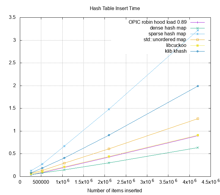
The insertion time is not as good as dense_hash_map under high load.
The reason is robin hood hashing moves the buckets around during the
insert, but dense_hash_map simply probe and insert it to an empty
bucket if found.
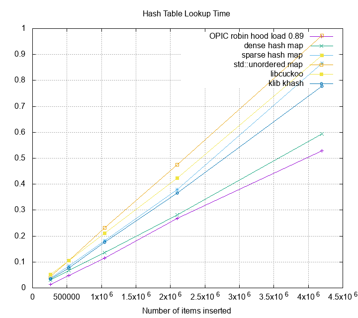
Luckily, robin hood hashing gets a faster lookup time compare to
dense_hash_map. I think the major reason is robin hood hashing
results a great expected probing number, and the overall throughput
benefits from it.
Hash table implementations has been focused on its speed over memory
usages. Turns out we can sacrifice some insertion time to gain way
better memory utilization, and also improve the look up time. I believe
this can be the new state of the art implementation for hash tables.
Let me know what you think in the comments. :)
Many details were omitted in this post, but will be discussed on my
next post. Some outlines for the things I’d like to cover would be
Probe distributions under different probing strategies (linear probing, quadratic probing, double hashing, and some probing methods I created).
Optimize probing by using gcc/clang vector extensions
Deletion mechanisms, its performance, and how it affects probe distributions.
Serialization and deserialization performance
Performance with different popular hash functions
Benchmark with other robin hood implementations
Benchmark with other embedded key-value store.
I may not be able to cover all the above in my next post, so please
put down your comment and let me know what do you want to read the most.
One more thing…
This robin hood hashing is implemented using my project
Object Persistence In C (OPIC). OPIC is a new general serialization
framework I just released. Any in-memory object created with OPIC can
be serialized without knowing how it was structured. Deserializing
objects from OPIC only requires one mmap syscall. That’s say, this
robin hood implementation can work not only in a living process, the
data it stored can be used as a key-value store after the process exits.
Right now, the throughput of OPIC robin hood hash map on small keys (6bytes)
is 9M (1048576/0.115454). This is way better than most
NoSQL key-value stores. The difference might come from
write ahead logs or some other IO? I’m not sure why the performance
gain is so huge. My next stop is to benchmark against other embedded
key-value store like rocksdb, leveldb and so forth.
References
If you’d like to know more about robin hood hashing, here are some
posts worth to read:
As people pointed out in hacker news and comment below, C++
std::string has 24 bytes overhead on small strings, so the memory
comparison is not fair. I’ll conduct another set of benchmarks using
integers tonight.
Also, one of the author of libcuckoo (@dga) pointed out that libcuckoo
would perform better if I use thread-unsafe version. I’ll also update
the benchmark with this new setup.
The short string problem brings up a question: what is the best
practice to use C++ hash map with short strings? Isn’t this a common
use case in daily programming? I tried to do some quick search but
didn’t find any useful information, and I’m suck at C++…
Any good idea on how to do this better?
]]><![CDATA[Autoconf Tutorial Part-3]]>2016-03-15T10:02:00-07:00http://www.idryman.org/blog/2016/03/15/autoconf-tutorial-part-3In this post I’ll show an example of how to write a cross-plaform OpenGL
program. We’ll explore more autoconf features, including config.h, third party
libraries, and many more.
Cross plaform OpenGL
Although OpenGL API is basically the same on all platforms, their headers and
linking options are very different on different plaforms! To use OpenGL on OSX,
you must include <OpenGL/gl.h>, however on other platform you have to use
<GL/gl.h>. Sometimes you might have multiple possible OpenGL implementation on
the same platform. If you search for OpenGL tutorials, most of it can only built
on one platform.
And that where autoconf comes to play its role. I recently submit a new version
of AX_CHECK_GL, that can address these complicated portability issues.
However, it doesn’t come with the default autoconf package, you need to include
the third party autoconf archive in your build script. Here’s how to
do it.
Adding Extra Macros
First, install third party macros by git submodule. Alternatively you can just
copy the macros you need, but be sure to include all the dependent macro it uses.
Next, in your configure.ac add the following line:
12
# before invoking AM_INIT_AUTOMAKEAC_CONFIG_MACRO_DIR([autoconf-archive/m4])
After these two steps you are free to invoke 500+ macros in the archive package.
C Preprocessor macros
Just adding the macro is not enough. You also have to pass the C preprocessor
macros to your C program. To do so, add another line to your configure.ac.
1
AC_CONFIG_HEADERS([config.h])
And now in your C program you can write the following to make it portable on all
systems. The listing is availabe in the AX_CHECK_GL document.
123456789101112
# include "config.h"#if defined(HAVE_WINDOWS_H) && defined(_WIN32)# include <windows.h>#endif#ifdef HAVE_GL_GL_H# include <GL/gl.h>#elif defined(HAVE_OPENGL_GL_H)# include <OpenGL/gl.h>#else# error no gl.h#endif
Wrapping it up
The full working example can be downloaded from here. Here is the
listing of each code:
configure.ac
12345678910111213141516171819
AC_INIT([gl-example], [1.0])AC_CONFIG_SRCDIR([gl-example.c])AC_CONFIG_AUX_DIR([build-aux])AC_CONFIG_MACRO_DIR([autoconf-archive/m4])AM_INIT_AUTOMAKE([-Wall -Werror foreign])AC_PROG_CC
AX_CHECK_GL
AX_CHECK_GLUT
# For glew you can simply use# AC_CHECK_LIB([GLEW], [glewInit])AC_CONFIG_HEADERS([config.h])AC_CONFIG_FILES([Makefile])AC_OUTPUT
The default rule for gl_example_SOURCES is to look at the c program with the
same name, thus can be omitted.
#include "config.h"#include <stdlib.h># if HAVE_WINDOWS_H && defined(_WIN32)#include <windows.h># endif#ifdef HAVE_GL_GL_H# include <GL/gl.h>#elif defined(HAVE_OPENGL_GL_H)# include <OpenGL/gl.h>#else# error no gl.h#endif# if defined(HAVE_GL_GLUT_H)# include <GL/glut.h># elif defined(HAVE_GLUT_GLUT_H)# include <GLUT/glut.h># else# error no glut.h# endifstaticvoidrender(void);intmain(intargc,char**argv){glutInit(&argc,argv);glutInitDisplayMode(GLUT_RGB|GLUT_DOUBLE);glutInitWindowSize(640,640);glutInitWindowPosition(100,100);glutCreateWindow("Hello World!");glutDisplayFunc(&render);glClearColor(0.0f,0.0f,0.0f,0.0f);glutMainLoop();return0;}voidrender(void){glClear(GL_COLOR_BUFFER_BIT|GL_DEPTH_BUFFER_BIT);glMatrixMode(GL_MODELVIEW);glLoadIdentity();glBegin(GL_TRIANGLES);glVertex3f(0.0f,0.0f,0.0f);glVertex3f(0.5f,1.0f,0.0f);glVertex3f(1.0f,0.0f,0.0f);glEnd();glutSwapBuffers();}
Try out the configure options by invoking ./configure --help. You’ll find it
provides rich options that is familiar to power users.
1234567891011121314151617181920212223
./configure --help
`configure' configures gl-example 1.0 to adapt to many kinds of systems.Usage: ./configure [OPTION]... [VAR=VALUE]......Optional Packages: --with-PACKAGE[=ARG] use PACKAGE [ARG=yes] --without-PACKAGE do not use PACKAGE (same as --with-PACKAGE=no) --with-xquartz-gl[=DIR] On Mac OSX, use opengl provided by X11/XQuartz instead of the built-in framework. If enabled, the default location is [DIR=/opt/X11]. This option is default to false.... PKG_CONFIG path to pkg-config utility PKG_CONFIG_PATH directories to add to pkg-config's search path
PKG_CONFIG_LIBDIR
path overriding pkg-config's built-in search path
GL_CFLAGS C compiler flags for GL, overriding configure script defaults
GL_LIBS Linker flags for GL, overriding configure script defaults
CPP C preprocessor
GLUT_CFLAGS C compiler flags for GLUT, overriding configure script defaults
GLUT_LIBS Linker flags for GLUT, overriding configure script defaults
So far I haven’t seen other build system that can do OpenGL cross platform
setup. (I only searched for CMake and Scons). Though autoconf is said to be
harder to learn, but by learning through these three articles, now the
syntax shouldn’t be that alien anymore, right?
In the next post, I’ll give another example of how to build a library, with unit
tests and debugger setup.
]]><![CDATA[Autoconf Tutorial Part-2]]>2016-03-14T16:28:00-07:00http://www.idryman.org/blog/2016/03/14/autoconf-tutorial-2This is the second post of the autoconf tutorial series. In this post I’ll cover
some fundamental units in autoconf and automake, and an example cross platform
X11 program that uses the concepts in this post. After reading this post, you
should be able to write your own build script for small scope projects.
Autoconf
Autoconf is part of the GNU Autotools build system. Autotools is a collection of
three main packages: autoconf, automake, and libtools. Each of the package has
smaller sub-packages including autoheader, aclocal, autoscan etc. I won’t cover
the details of all the packages; instead I’ll only focus on how autoconf plays
its role in the build chain.
Autoconf is mainly used to generate the configure script. configure is a
shell script that detects the build environment, and output proper build
flags to the Makefile, and preprocessor macros (like HAVE_ALLOCA_H) to
config.h. However, writing a good portable, extensible shell script isn’t
easy. This is where the gnu m4 macro comes in. Gnu m4 macro is an
implementation of the traditional UNIX macro processor. By using m4, you can
easily create portable shell script, include different pre-defined macros, and
define your own extensions easily.
In short, autoconf syntax is shell script wrapped by gnu m4 macro.
In the early days, writing portable shell scripts wasn’t that easy. For example
not all the mkdir support -p option, not all the shells are bash
compatible, etc. Using the m4 macro to perform the regular shell logics, like
AS_IF instead if if [[ ]]; then..., AS_MKDIR_P instead of mkdir -p,
AS_CASE instead of case ... esac makes your configure script works better on
all unix/unix-like environment, and more conventional. Most of the time you’ll
be using macros instead of bare bone shell script, but keep in mind that behind
the scene your final output is still shell script.
M4 Macro Basics
Though the first look at M4 macros is very alien and unfriendly, but it only
consist two basic concepts:
Macro expansion
Quoting
You can define a macro like so:
1234567
# define a macro MY_MACRO that expands to text ABCm4_define([MY_MACRO], [ABC])MY_MACRO=> ABC
# define a macro that is visible to other m4 scriptsAC_DEFUN([MY_MACRO], [ABC])MY_MACRO=> ABC
It’s pretty much similar to C macro or Lisp macro. The macro expands at compile
time (configure.ac => configure). You can define a macro MY_MACRO that
expands to a snippet of shell script. Here we just expands it to ABC, which
doesn’t have any meaning in shell script and can trigger an error.
Every symbol in your script is expandable. For example if you simply write ABC
in your script, is it a shell symbol, or is it a m4 symbol that needs to expand?
The m4 system uses quoting to differentiate the two. The default quoting in
autoconf is square brackets [, ]. Though you can change it, but it is highly
unrecommended.
12
ABC # m4 would try to find *macro* definition of ABC and try to expand it[ABC]# shell symbol ABC
Why does it matter? Consider these two examples
123456789
ABC="hello world"# m4 would try to expand ABC, hello, and world[ABC="hello world"]# m4 would just produce ABC="hello world" to the output# m4 will expand MY_MACRO and BODY *before* defining MY_MACRO as a symbol to# BODY.AC_DEFUN(MY_MACRO, BODY)# safeAC_DEFUN([MY_MACRO], [BODY])
This is the base of all m4 macros. To recap, always quote the arguments for
the macros, including symbols, expressions, or body statements. (I skipped
some edge cases that requires double quoting or escapes, for the curious please
check the autoconf language).
Printing Messages
Now we know the basic syntax of m4, let’s see what are the functions it
provides. In the configure script, if you invoke echo directly the output
would be redirected to different places. The convention to print message in
autoconf, is to use AC_MSG_* macros. Here are the two macros that is most
commonly used:
12345
# Printing regular messageAC_MSG_NOTICE([Greetings from Autoconf])# Prints an error message and stops the configure scriptAC_MSG_ERROR([We have an error here!]
For the more curious, check the Printing Messages section in autoconf
manual.
If-condition
To write an if condition in autoconf, simply invoke
AS_IF(test-1, [run-if-true-1], ..., [run-if-false]).
The best way to see how it works is by looking an example:
12345678910111213141516171819202122
abc="yes"def="no"AS_IF([test"X$abc"="Xyes"], # test condition[AC_MSG_NOTICE([abc is yes])], # then case[test"X$def"="Xyes"], # else if[AC_MSG_NOTICE([def is yes])],
[AC_MSG_ERROR([abc check failed])]# else case)# expands to the following shell scriptabc="yes"def="no"if test"X$abc"="Xyes"; then :
# test condition$as_echo"$as_me: abc is yes" >&6
elif# then casetest"X$def"="Xyes"; then :
# else if$as_echo"$as_me: def is yes" >&6
elseas_fn_error $?"abc check failed"# else casefi
Note that we don’t use common shell test operator [[ and ]], instead we use
test because the square bracket is preserved for macro expansion. The
recommended way to invoke test is test "X$variable" = "Xvalue". This is how we
avoid null cases of the shell variable.
Another common branching function is AS_CASE(word, [pattern1], [if-matched1], ..., [default])
the logic is pretty much the same.
That all the basics we need to know for autoconf, let’s take a break and switch
to automake.
Automake
Like autoconf, automake is additional semantics on top of another existing
language – the Makefile syntax. Unlike autoconf, it’s not using m4 to extend
the syntax. It uses a naming convention that converts to the actual logic. Most
of the time, we only need to use the following two rules, which we’ll discuss in
detail.
where_PRIMARY = targets
target_SECONDARY = inputs
where_PRIMARY = targets
This syntax has three parts, targets, type PRIMARY, and where to install
where. Some examples shown as below:
12345
# target "hello" is a program that will be installed in $bindirbin_PROGRAMS= hello
# target "libabc" is a library that will be installed in $libdirlib_LIBRARIES= libabc.la
The targets is a list of targets with the type PRIMARY. Depending on what
PRIMARY is, it can be a program, a library, a shell script, or whatever
PRIMARY supports. The current primary names are “PROGRAMS”, “LIBRARIES”,
“LTLIBRARIES”, “LISP”, “PYTHON”, “JAVA”, “SCRIPTS”, “DATA”, “HEADERS”, “MANS”,
and “TEXINFOS”.
There are three possible type of variables you can put into the where clause.
GNU standard directory variables (bindir, sbindir, includedir, etc.) omitting
the suffix “dir”. See GNU Coding Standard - Directory Variables for
list of predefined directories. Automake extends this list with pkgdatadir,
pkgincludedir, pkglibdir, and pkglibexecdir Automake will check if your
target is valid to install the directory you specified.
Self-defined directories. You can hack around automake default type check by
defining your own directories. Do not do this unless you have a good reason!
123456
# Work around forbidden directory combinations. Do not use this# without a very good reason!my_execbindir=$(pkglibdir)my_doclibdir=$(docdir)my_execbin_PROGRAMS= foo
my_doclib_LIBRARIES= libquux.a
Special prefixes noinst_, check_, dist_, nodist_, nobase_, and
notrans_. noinst_ indicates the targets that you don’t want to install;
check_ is used for unit tests. For the others are less common, please check
the automake manual for detail.
target_SECONDARY = inputs
Depending on what your PRIMARY type is, there are different SECONDARY types
you can use for further logic. The common SECONDARY types are
_SOURCES defines the source for primary type _PROGRAMS or _LIBRARIES
_CFLAGS, _LDFLAGS, etc. compiler flags used for primary type _PROGRAMES
or _LIBRARIES
Note that the invalid character in target name will get substituted with
underscore. The following example illustrate all the above:
1234
lib_LTLIBRARIES= libgettext.la
# the dot got substituted with underscorelibgettext_la_SOURCES= gettext.c gettext.h
include_HEADERS= gettext.h
The example above requires libtool. You need to declare
AC_PROG_LIBTOOL in your configure.ac for it to work.
Wraps it up - A X11 example program
With everything we learnt so far, let’s write a more complicated autoconf
program. This is a very simple X11 program that aims to be portable on all
existing platforms with valid X11 installed. To test if X11 is installed, we use
the macro AC_PATH_XTRA, the manual for this macro is defined in
autoconf existing test for system services.
The manual says: An enhanced version of AC_PATH_X. It adds the C compiler flags
that X needs to output variable X_CFLAGS, and the X linker flags to X_LIBS.
Define X_DISPLAY_MISSING if X is not available. And in the AC_PATH_X it
states “If this method fails to find the X Window System … set the shell
variable no_x to ‘yes’; otherwise set it to the empty string”. We can use the
logic and write our configure.ac script as following:
123456789101112131415161718192021222324
AC_INIT([x11-example], [1.0])# safety check in case user overwritten --srcdirAC_CONFIG_SRCDIR([x11-example.c])AC_CONFIG_AUX_DIR([build-aux])AM_INIT_AUTOMAKE([-Wall -Werror foreign])# Check for C compilerAC_PROG_CC
# Check for X11# It exports variable X_CFLAGS and X_LIBSAC_PATH_XTRA
# AC_PATH_XTRA doesn't error out by default,# hence we need to do it manuallyAS_IF([test"X$no_x"="Xyes"],
[AC_MSG_ERROR([Could not find X11])])AC_CONFIG_FILES([Makefile])AC_OUTPUT
Note that the AC_PATH_XTRA export variables X_CFLAGS and X_LIBS. To use
these variables in Makefile.am, just surround it with @.
1234567
bin_PROGRAMS= x11-example
x11_example_SOURCES= x11-example.c
x11_example_CFLAGS= @X_CFLAGS@
# AX_PATH_XTRA only specify the root of X11# we still have to include -lX11 ourselvesx11_example_LDFLAGS= @X_LIBS@ -lX11
That all we need to build a platform independent X11 program! Check the full
source on github. The X11 example program was written by Brian Hammond
2/9/96. He generously released this to public for any use.
This program can easily work on Linux. I’ll use OSX as an example of how cross
platform works. Before you run the example, make sure you have
XQuartz installed.
12345
cd example-2
autoreconf -vif # shortcut of --verbose --install --force./configure --with-x --x-includes=/opt/X11/include/ --x-libraries=/opt/X11/lib
make
./x11-example
Change the --x-includes and --x-libraries to proper directory if you
installed the xquartz to a different location.
I only introduced very little syntax for autoconf (if-else, print message) and
automake (primary/secondary rules, use of export variables by @). But just
using these basic component is already very sufficient for writing conventional
build scripts. How to do it? Check the [existing tests provided by
autoconf][exsisting test]. Here are some of the most commonly used existing
checks:
For the checks that are not included in the default autoconf package, it
probably exists in the extended package autoconf archive, which I’ll
cover in the next post.
]]><![CDATA[Autoconf Tutorial Part-1]]>2016-03-10T14:55:00-08:00http://www.idryman.org/blog/2016/03/10/autoconf-tutorial-1It’s been more than a year since my last update to my blog. I learnt a lot new
stuffs in last year, but was too busy on work to write down what I’ve learnt.
Luckily I got some breaks recently, and I’ll pick up some of the posts that
I’ve wanted to write about. First I’ll start with a autoconf tutorial series.
This is one of the difficult material to learn, but I’ll try to re-bottle it
to make it more accessible to everyone.
What is Autoconf?
If you have ever installed third party packages, you probably already used the
result of autoconf. Autoconf, automake, and libtool are the GNU Autotools
family that generate the installation script:
123
./configure
make
make install
Many unix or unix-like system make use of the simplicity of these installation
steps. The linux distros usually provides custom command line options to the
./configure to customize the build, and further repackage it with rpm or dpkg.
Autoconf is not only a build system, it also does many system compatibility
checks. Does your operating system support memory-mapped file? Does your
environment has X11? The standard autoconf already support a wide variety of
checks, and there are 500 more in Autoconf Archive. It’s the defacto
standard build standard for building small and large linux/unix programs.
Though the output of autoconf is easy for user to install, writing autoconf
build script is less intuitive, compare to other fancier solution like
CMake or Scons. And that’s why I’m writing this tutorial - to
reduce the learning curve of using autoconf.
Through out this series, I’ll start with a minimal autoconf project, and later
introduce how to bring in debug setup, how to build a library, how to setup unit
test, how to write your own cross platform checks etc.
Hello Autoconf
The best way to learn is to practice through examples. Let’s start with a very
simple one. First create a directory holding your project,
12
$ mkdir example-1
$ cd example-1
Install the autoconf on your system if it wasn’t installed
And create three files: configure.ac, Makefile.am, and the program itself
hello.c.
configure.ac
12345678910111213141516171819202122232425262728
# Must init the autoconf setup# The first parameter is project name# second is version number# third is bug report addressAC_INIT([hello], [1.0])# Safety checks in case user overwritten --srcdirAC_CONFIG_SRCDIR([hello.c])# Store the auxiliary build tools (e.g., install-sh, config.sub, config.guess)# in this dir (build-aux)AC_CONFIG_AUX_DIR([build-aux])# Init automake, and specify this program use relaxed structures.# i.e. this program doesn't follow the gnu coding standards, and doesn't have# ChangeLog, COPYING, AUTHORS, INSTALL, README etc. files.AM_INIT_AUTOMAKE([-Wall -Werror foreign])# Check for C compilerAC_PROG_CC
# We can add more checks in this section# Tells automake to create a Makefile# See https://www.gnu.org/software/automake/manual/html_node/Requirements.htmlAC_CONFIG_FILES([Makefile])# Generate the outputAC_OUTPUT
That’s the minimal build script you need for your first autoconf program.
Let’s try what we’ve got with this setup. Make sure your are in the example-1
directory.
123456789101112131415161718192021
# this creates the configure script$ autoreconf --verbose --install --force
$ ./configure --help
$ ./configure
ecking for a BSD-compatible install... /usr/bin/install -c
checking whether build environment is sane... yes
checking for a thread-safe mkdir -p... build-aux/install-sh -c -d
checking for mawk... no
...
config.status: creating Makefile
config.status: executing depfiles commands
# Now try the makefile$ make
gcc -DPACKAGE_NAME=\"hello\" -DPACKAGE_TARNAME=\"hello\" -DPACKAGE_VERSION=\"1.0\" -DPACKAGE_STRING=\"hello\ 1.0\" -DPACKAGE_BUGREPORT=\"\" -DPACKAGE_URL=\"\" -DPACKAGE=\"hello\" -DVERSION=\"1.0\" -I. -g -O2 -MT hello.o -MD -MP -MF .deps/hello.Tpo -c -o hello.o hello.c
mv -f .deps/hello.Tpo .deps/hello.Po
gcc -g -O2 -o hello hello.o
# We now have the hello program built$ ./hello
hello world!
# Create hello-1.0.tar.gz that contains the configure script$ make dist
You might think this is overkill for a hello world program, but you can also
think in another way. Just adding the configure.ac and Makefile.am made a
simple hello world program looks like a serious production ready project (with
all these fancy configure checks and compiler flags).
Let’s iterate through each of the build script.
configure.ac
The syntax for configure.ac is MACRO_NAME([param-1],[param-2]..). The
parameter passed to the macro must be quoted by square brackets, (unless it is
another macro that you want to expand BEFORE calling the outer macro, which is
very rare). The macros will expands to shell script that perform the actual
checks. You can also write shell script in your configure.ac file. Just one
difference, you should use if test <expression>; then... instead of
if [[ <expression> ]]; then... for condition branching, because the square
brackets would get expanded by the autoconf macro system.
AC_INIT(package, version, [bug-report], [tarname], [url]) In every autoconf
configure script, you must first initialize autoconf with this macro. The
square braket that wraps around each parameter cannot be omitted.
AC_CONFIG_SRCDIR(dir) Next we specify a unique file identifying we are in
the right directory. This is a safety check in case user override the –srcdir
command line option.
AC_CONFIG_AUX_DIR(dir) By default autoconf will create many auxiliary files
that help to build and distribute the programs. However we don’t want to have
these files to mess up the project home directory. In convention we call this
macro with [build-aux] so that it put these extra files in build-aux/
instead of project home.
AM_INIT_AUTOMAKE([options]) Initializes automake. An important note here is
in early phase of your project development, you probably want to provide the
option foreign to init automake. If foreign wasn’t provided, automake will
complain that your project didn’t confirm to gnu coding standards, which would
require you to have README, ChangLog, AUTHORS, and many other files in your
project’s home directory.
AC_PROG_CC Checks for a valid C compiler. There are hundreds more checks you
can put in this section.
AC_CONFIG_FILES(files) Required by automake to create the output file. Here
we simply put the Makefile in. Checks the automake documentation for more
detail.
automake.
AC_OUTPUT Creates the configure script
Makefile.am
The automake file Makefile.am is an extension to Makefile. You can write
standard make syntax, but normally you only need to define variables that
conforms to the uniform naming scheme. In this post I’ll only give
rough explanation, and dive in more detail in next post.
bin_PROGRAMS = hello The output is a PROGRAM (other options are LIBRARY,
HEADER, MAN, etc.) named hello, and will be installed in bin directory
(default to /usr/local/bin, but can be configured when invoking
./configure.
hello_SOURCES = hello.c The sources of hello program is hello.c
The complete program can be found in my github repository:
Example 1.
More make targets
The Makefile generated by Autoconf and automake has more commands that you can
run:
make all
Build programs, libraries, documentation, etc. (same as make).
make install
Install what needs to be installed, copying the files from the package’s tree to system-wide directories.
make install-strip
Same as make install, then strip debugging symbols. Some users like to trade space for useful bug reports…
make uninstall
The opposite of make install: erase the installed files. (This needs to be run from the same build tree that was installed.)
make clean
Erase from the build tree the files built by make all.
make maintainer-clean
Erase files that generated by autoconf.
make distclean
Additionally erase anything ./configure created.
make check
Run the test suite, if any.
make installcheck
Check the installed programs or libraries, if supported.
make dist
Recreate package-version.tar.gz from all the source files.
When I first survey what build system I should pick for my own projects, I often
see other alternatives claiming autoconf is old and hard to use. This is
partially true, but the more I dig in the more I found how powerful autoconf is.
As you see, this example can already cover many common cases, with a succinct
build script and very powerful output. The package created by make dist
only requires a minimal unix compatible environment (shell and make) to run.
In the next post I’ll cover more detail in the autoconf syntax and Automake
syntax.
]]><![CDATA[Writing 64 bit assembly on Mac OS X]]>2014-12-02T17:18:00-08:00http://www.idryman.org/blog/2014/12/02/writing-64-bit-assembly-on-mac-os-xMany assembly tutorials and books doesn’t cover
how to write a simple assembly program on the Mac OS X.
Here are some baby steps that can help people who
are also interested in assembly to get started
easier.
Mach-O file format
To get started on writing OSX assembly, you need to
understand OSX executable file format – the Mach-O
file format. It’s similar to ELF, but instead
of sections of data, bss, and text, it has segments that
contains sections.
A common assembly in Linux like
123
.sectiondata.sectiontext# your code here
would translate into this in Mach-O
123456
.section__DATA,__data# __DATA is segment, __data is section.section__TEXT,__text# __TEXT is segment, __text is section# your code here
Mach-O is pretty flexible. You can embed a
cstring section in your __TEXT segment instead
of putting it in __DATA,__data. Actually this is
the default behavior that compiler does on your Mac.
Hello Assembly
Now we know how to translate common linux assembly
to mac, let’s write a basic program – do a system call
with an exit code.
On x86 you do a system call by int x80 instruction. On
64 bit machine, you do this by syscall. Here’s the sample
code:
1234567
# Simple exit program.section__TEXT,__text.globl_main_main:movl$0x2000001,%eax# system call $1 with $0x2000000 offsetmovl$0,%ebx# set the exit code to be $0syscall
you can compile the code by the following commands:
1234
as exit.s -o exit.o
ld exit.o -e _main -o exit# -e specify the entry point of the executable./exit
echo$?# show last return code, should show 0
To perform a system call, you put the system call number in
%eax, and put the actual exit code to %ebx. The system
call number can be found in /usr/include/sys/syscall.h.
The system call number need to add an offset 0x2000000, because
OSX has 4 different class of system calls. You can find the reference
here XNU syscall.
System call by using wrapper functions
If you’re like me that had no assembly background, you might
feel that syscall is alien to you. In C, we usually use
wrapper functions to perform the call:
123456789101112
# exit2.s# To compile it, type the following in shell# as exit2.s -o exit2.o# ld exit2.o -e _main -lc -o exit.section__TEXT,__text.globl_main_main:pushq%rbpmovq%rsp,%rbpmovl$5,%edi# exit(5);callq_exit
Now we call a libc function instead of performing a system
call. To do this we need to link to libc by passing -lc
to linker ld. There are several things you need to do
to make a function call.
Call frame
We need to prepare the stack before we call a function. Else
you would probably get a segmentation fault.
The values in %rsp and %rbp is used to preserve frame information.
To maintain the stack, you first push the base register %rbp
onto the stack by pushq %rbp;
then you copy the stack register %rsp to the base register.
If you have local variables, you subtract %rsp for space.
Remember, stack grows down and heap grows up.
When releasing the frame, you add the space back to %rsp.
A live cycle of a function would look like this:
123456789
# function startpushq%rbpmovq%rsp,%rbpsubq$4,%rsp# reserve 4 bytes on stackmovl$5,-4(%rbp)# We usually use base register instead# of stack pointer to access dataaddq$4,%rsp# release the stackpopq%rbp# restore old %rbpretq# function ends
The stack size can be set at link time. On OSX, below are the
example parameters you can pass to ld to set the stack size:
Although the AMD64 architecture uses 64-bit pointers, implementations
are only required to handle 48-bit addresses. Therefore, conforming processes may only
use addresses from 0x00000000 00000000 to 0x00007fff ffffffff
I don’t know a good answer of how to chose a good stack address.
I just copy whatever a normal code produces.
If the class is MEMORY, pass the argument on the stack.
If the size of an object is larger than four eight bytes, or
it contains unaligned fields, it has class MEMORY.
If the class is INTEGER, the next available register of the sequence %rdi,
%rsi, %rdx, %rcx, %r8 and %r9 is used.
If the class is SSE, the next available vector register is used, the registers
are taken in the order from %xmm0 to %xmm7.
The exit() function only need one integer parameter, therefore we put
the exit code in %edi. Since the parameter is type int, we use 32 bit
variance of register %rdi and the instruction is movl (mov long) instead
of movq (mov quad).
Hello world
Now we know the basics of how to perform
a system call, and how to call a function.
Let’s write a hello world program.
12345678910111213141516171819
# hello_asm.s# as hello_asm.s -o hello_asm.o# ld hello_asm.o -e _main -o hello_asm.section__DATA,__datastr:.asciz"Hello world!\n".section__TEXT,__text.globl_main_main:movl$0x2000004,%eax# preparing system call 4movl$1,%edi# STDOUT file descriptor is 1movqstr@GOTPCREL(%rip),%rsi# The value to printmovq$100,%rdx# the size of the value to printsyscallmovl$0,%ebxmovl$0x2000001,%eax# exit 0syscall
The global variable str can only be accessed through GOT
(Global Offset Table). And the GOT needs to be access from
the instruction pointer %rip. For more curious you can
read Mach-O Programming Topics: x86-64 Code Model.
The register used for syscall parameters are a little
bit different than the normal function call.
It uses %rdi, %rsi, %rdx, %r10, %r8 and %r9.
You cannot pass more than 6 parameters in syscall, nor
can you put the parameters on the stack.
Hello world using printf
Now you know the basics of assembly. A hello world
example using printf should be trivial to read:
The 64 bit assembly looks more vague than the tutorials
written in X86 assembly. Once you know these basic differences,
it’s easy for you to learn assembly in depth on your own,
even if the material is designed for x86. I highly recommend
the book “Programming from the ground up”. It is well written
for self study purpose.
]]><![CDATA[Integer Promotion Part 2]]>2014-11-29T18:34:00-08:00http://www.idryman.org/blog/2014/11/29/integer-promotion-part-2It’s been a while since I wrote my last article. I recently read an old book Expert C Programming and found there are many C langauge details that I never think about. Review and rethink what C integer promotion rules meant to C is one of the interesting topic that I want to share with you.
What is type systems?
Type is the methods that interpret and process your data.
Sounds familiar to OOP? Definiing a class IS defining a method.
In C, expressions on different data type produces different
instructions. What instruction to generate? Depends on the data
type. (int is different than float, for example).
A chunk of data in memory or register can mean anything
on a CPU. The type system defines how operators works on different types.
Given the example below:
123456
int*p=0x00007ffffffffcc0;inti=1;int*q=p+i;// => 0x00007fffffffffcc4 because the type "pointer to int"// defines the multiplier of the offset is 4int*r=p+q;// Invalid in C type system.
When adding an integer to a pointer, the compiler knows the offset multiplier
by the type of the pointer points to. If p where defined as char* p, then
the multiplier would be 1. Also, the + operator only make sense to add an
offset to a pointer, therefore adding two pointer together is invalid in C
syntax.
Review C integer promotion rules
I wrote an article about C integer promotion 2 years ago: Deep C: Integer Promotion. The standard integer promotion rules in C99 is listed below.
If an int can represent all values of the original type, the value is converted
to an int; otherwise, it is converted to an unsigned int. These are called the
integer promotions. All other types are unchanged by the integer promotions.
This is called value preserving. On machine level, the arithmetic works best on
a whole register (or 32 bit register). Remember that C’s philosophy is to make
your program runs as fast as possible, so it loads your small data chunk into
the whole register, then do the calculation.
However, things worked differently on K&R C. It’s was defined as unsigned
preserving. When mixing a signed and unsigned integer, the result is unsigned
type. Below is the example copied from Expert C Programming book.
12345
if(-1<(unsignedchar)1){printf("C dialect after ANSI C, including C89, C99, and after\n");}else{printf("Pre ANSI C (K&R) dialect. -1 is treated as unsigned value 0xFFFFFFFF and thus greater than 1 ! \n");}
Mixing unsigned and signed integer in modern C
Although most of the time C will preserve the value of the type for you,
you can still get surprising result. When the signed integer can’t hold
the unsigned value, everything is converted to unsigned integer.
123456
if(-1<sizeof(int)){printf("-1 is less than 4\n");}else{printf("-1 is treated as 0xffffffff. Because sizeof returns size_t which is an unsigned int\n");}return0;
This program will execute the else branch and print:
Always be careful when you mix unsigned and signed integer in expressions.
When possible, type cast it to signed int. C is designed to make program fast,
but not safe for beginners. Additional checks would create a lot of overhead
in the runtime, so the developer need to know the system and language well
to avoid shooting at their own foot. Another possible reason may be that
the original C developers were all operating system writers and compiler
writers. Therefore, the mappings between Assembly and C langauge is
straight forward to them.
]]><![CDATA[Introducing Hadoop-FieldFormat]]>2014-03-06T14:25:00-08:00http://www.idryman.org/blog/2014/03/06/introducing-hadoop-fieldformatHadoop FieldFormat is the new library I released that is flexible and robust for reading and setting schema information in Hadoop map-reduce program. We use this library to record the meta information for the data, and improve the semantic when building large map-reduce pipe-lined tasks. The project is quite stable now and we already used it in our production system. Any suggestion is welcome!
The problem
The map-reduce architecture is really good at aggregating large dataset and ad-hoc perform computation; however, when the number dataset increases, it becomes difficult to manage the meta data of those dataset. The biggest issue is data by default is semi-structured; there’s no schema or header information to tell you the semantic of the data. When working in raw map-reduce, this is typical code that I write:
There’s no semantic associated with the data, so you can only hard code the semantic and hope the fields order will stay the same forever. If the upstream process inserted a new field to this dataset, your program may still run, but produce wrong result that might be difficult to catch by downstream program.
The same issue happens in Pig and cascading too. Pig, for example:
If the input format changed, you’ll need to be very careful to make sure all the downstream process are corrected. Moreover, if you want to run map-reduce across different versions of dataset, you may not be able to run it because the order of the fields is different!
Hive and HCatalog
Goal: lightweight semantic attached to the data
Eat our own dog food – introducing Hadoop FieldFormat!
You may be surprised by how simple the solution is. First, answer this:
Where does hadoop store the meta data for map-reduce jobs? _logs.
What hadoop FieldFormat does is reading and writing header.tsv. Also, provides
a convenient API in java to access the data field using the java Map interface.
]]><![CDATA[Hadoop performance tuning best practices]]>2014-03-05T11:17:00-08:00http://www.idryman.org/blog/2014/03/05/hadoop-performance-tuning-best-practicesI have been working on Hadoop in production for a while. Here are some of the performance tuning tips I learned from work. Many of my tasks had performance improved over 50% in general. Those guide lines work perfectly in my work place; hope it can help you as well.
Tuning Hadoop run-time parameters
Hadoop provides a set of options on cpu, memory, disk, and network for performance tuning. Most hadoop tasks are not cpu bounded, what we usually look into is to optimize usage of memory and disk spills.
Memory tuning
The general rule for memory tuning is: use as much memory as you can, but don’t trigger swapping. The parameter you can set for task memory is mapred.child.java.opts. You can put it in your configuration file.
You can tune the best parameters for memory by monitoring memory usage on server using Ganglia, Cloudera manager, or Nagios. Cloudera has a slide focused on memory usage tuning, the link is here
Minimize the map disk spill
Disk IO is usually the performance bottleneck. There are a lot of parameters you can tune for minimizing spilling. What I use the most are:
Although you can further tune reducer buffer, mapper sort record percent, and various of stuff, I found the best thing to do is reduce the mapper output size. Most of the time, the performance is fast enough after I refactor the mapper to output as little data as possible. For more information, check the same cloudera’s performance tuning guide.
Tuning mapper tasks
Unlike reducer tasks which you can specify the number of reducer, the number of mapper tasks is set implicitly. The tuning goal for the mapper is control the amount of mapper and the size of each job. When dealing with large files, hadoop split the file in to smaller chunk so that mapper can run it in parallel. However, the initializing new mapper job usually takes few seconds, this is also a overhead that we want to minimize. These are the things you can do:
Reuse jvm task
If the average mapper running time is shorter than one minute, you can increase the mapred.min.split.size, so that less mappers are allocated in slot and thus reduces the mapper initializing overhead.
Use Combine file input format for bunch of smaller files. I had an implementation that also use mapred.min.split.size to implicitly control the mapper size. You can find the project on github. The explanation of the project can be found on my blog.
Use configuration file and command line arguments to set parameters
When I first started on hadoop, I setup those parameters in java program, but it is so hard-coded and inflexible. Thankfully, hadoop provides Tool interface and ToolRunner class to parse those parameters for you. Here’s a sample program:
123456789101112
publicclassExampleJobextendsConfiguredimplementsTool{publicstaticvoidmain(String[]args)throwsException{System.exit(ToolRunner.run(newExampleJob(),args));}publicintrun(String[]args)throwsException{Configurationconf=getConf();Jobjob=newJob(conf);// configure the rest of the job}}
If your main class implements the interface, your program can take the config file as input:
1
hadoop jar ExampleJob-0.0.1.jar ExampleJob -conf my-conf.xml arg0 arg1
You can even pass extra parameters through command line like this:
1
hadoop jar ExampleJob-0.0.1.jar ExampleJob -Dmapred.reduce.tasks=20 arg0 arg1
Setting configuration as run-time arguments make you easier to test different parameters without recompile the program.
Tuning application-specific performance
Beyond general hadoop parameter setup, you can optimize your map-reduce program using some small tricks. Here are the tricks that I used the most.
Minimize your mapper output
Recall that mapper spill size is a serious performance bottleneck. The size of mapper output is sensitive to disk IO, network IO, and memory sensitive on shuffle phase. Minimizing the mapper output can improve the general performance a lot.
To do this, you can try the following
Filter out records on mapper side, not on reducer side.
Use minimal data to form your map output key and map output value.
Extends BinaryComparable interface or use Text for your map output key
Set mapper output to be compressed
Above all the optimization tips, I found this make the biggest change to many of my tasks, unless I can’t find a smaller key to reduce the mapper output.
Balancing reducer’s loading
Another common performance issue that you might encounter is unbalanced reducer tasks: one or several reducer takes most of the output from mapper and ran extremely long compare to other reducers.
To solve this, you can either
Implement a better hash function in Partitioner class.
If you know what keys are causing the issue, you can write a preprocess job to separate keys using MultipleOutputs. Then use another map-reduce job to process the special keys that cause the problem.
Conclusion
It’s fun to write raw map-reduce jobs because it gives you more precise control over performance tuning. If you already experienced hive or pig, I encourage you to try how to optimize the same job using raw map-reduce. You can find a lot of performance gain and more space to tune the performance. For more curious, you can also check the Yahoo’s tuning hadoop performance guides.
]]><![CDATA[Setting up Jasper Server on Linux]]>2014-02-26T13:26:00-08:00http://www.idryman.org/blog/2014/02/26/setting-up-jasper-server-on-linuxJasper is one of the standard report generator in the industry. However, setting up Jasper is a pain of ass. This post is my note for setting up Jasper on Linux, in case I have to do it again in the future…
Setting up an Ubuntu instance on Amazon
The first thing you need to do when you launch an Amazon EC2 instance is add the hostname to hosts. Copy /etc/hostname to /etc/hosts like so:
1
127.0.0.1 localhost ip-10-0-0-1
The ip-10-0-0-1 is the host name in your /etc/hostname. You’ll need this setup else the jasper installation script might fail.
This section is referenced to Jaspersoft wiki. We found that when selecting query language as plsql, jasperserver rejects the uploaded report.
To solve the issue, you’ll need to extend jasperserver with this plugin: jasperreports-extensions-3.5.3.jar. Download the jar, and place it to /opt/jasperreports-server-cp-5.5.0/apache-tomcat/webapps/jasperserver/WEB-INF/lib/.
Now, cd to /opt/jasperreports-server-cp-5.5.0/apache-tomcat/webapps/jasperserver/WEB-INF, and add one line to classes/jasperreports.properties.
Edit applicationContext.xml. Search for supportedQueryLanguages and change it to the following.
1234567891011121314151617181920212223242526272829
<beanclass="com.jaspersoft.jasperserver.api.engine.jasperreports.util.DataSourceServiceDefinition"><propertyname="serviceBeanName"value="jdbcDataSourceServiceFactory"/><propertyname="supportedQueryLanguages"><set><value>sql</value><value>SQL</value><!-- Add these two value lines for the Oracle PL/SQL Language --><value>plsql</value><value>PLSQL</value></set></property></bean><beanclass="com.jaspersoft.jasperserver.api.engine.jasperreports.util.DataSourceServiceDefinition"><propertyname="serviceBeanName"value="jndiJdbcDataSourceServiceFactory"/><propertyname="supportedQueryLanguages"><set><value>sql</value><value>SQL</value><!-- Add these two value lines for the Oracle PL/SQL Language --><value>plsql</value><value>PLSQL</value></set></property></bean>
More specifically, tomcat’s memory usage. The default memory setting is quite low and jasper is pretty in-responsive to user clicks. To change the setting, edit /opt/jasperreports-server-cp-5.5.0/apache-tomcat/scripts/ctl.sh and change the two JAVA_OPTS to
Relaunch your jasper server again. Now it should run more smoothly.
Conclusion
ITS A PAIN TO RUN JASPER…
Thanks to all the people that wrote wiki and articles to help me out. I hope I’ll never need to set it up again.
]]><![CDATA[Capture path info in hadoop InputFormat class]]>2014-01-27T15:11:00-08:00http://www.idryman.org/blog/2014/01/27/capture-path-info-in-hadoop-inputformat-classOn the last post I presented how to use Mapper context object to obtain Path information. This is a nice way to hack for ad-hoc jobs; however, it’s not really reusable and abstract. In this post, I’ll show you how to subclass Text, TextInputFormat, and LineRecordReader and create reusable components across all of your hadoop tasks.
Input WorkFlow
Before we go through all the classes, let me show you how hadoop read the files in.
By default, hadoop uses TextInputFormat, which inherits FileInputFormat, to process the input files.
TextInputFormat allocates LineRecordReader and passed it to Task runtime.
Task first initiates LineRecordReader, then wrap the LineRecordReader into Context object.
In Mapperrun methods, it calls the method nextKeyValue() in Context, and reads the LongWritable key from context.getCurrentKey() and Text value from context.getCurrentValue(). Those methods delegates to LineRecordReader’s methods nextKeyValue(), getCurrentKey(), and getCurrentValue().
Finally, Mapper passes the key-value pair to map method that we usually overrides.
In order to put the path information into this workflow, we can extend the Text class and put the path information into it. To make this work, we need to create three new classes: TextWithPath, TWPInputFormat, and TWPRecordReader.
TextWithPath.java
Here is our content wrapper – TextWithPath. It doesn’t do much; there’s a new constructor which accepts Path, and there’s a getter method to get Path.
The new TWPInputFormat is almost identical to TextInputFormat, except it uses TextWithPath instead of Text, and the createRecordReader method returns TWPRecordReader instead of LineRecordReader.
Finally, in the TWPRecordReader, this is where I put my logic in. In the initialize method, you can get the FileSplit and get the Path object out of it. Next, let’s override nextKeyValue, and updates the value on every call. Lastly, remember to override getCurrentValue(), else it will only return parent’s value (Text), not the value with TextWithPath class.
Here is a demo code to test the output. In addition to normal map reduce tasks, we set the input format class to TWPInpuFormat; on the Mapper side, we expect the input is TextWithPath, not Text. The whole program can be downloaded from this github repo. Hadoop TextWithPath
packageorg.idryman;importjava.io.IOException;importorg.apache.hadoop.conf.Configuration;importorg.apache.hadoop.conf.Configured;importorg.apache.hadoop.fs.Path;importorg.apache.hadoop.io.IntWritable;importorg.apache.hadoop.io.LongWritable;importorg.apache.hadoop.io.NullWritable;importorg.apache.hadoop.io.Text;importorg.apache.hadoop.mapreduce.Job;importorg.apache.hadoop.mapreduce.Mapper;importorg.apache.hadoop.mapreduce.lib.output.FileOutputFormat;importorg.apache.hadoop.mapreduce.lib.reduce.IntSumReducer;importorg.apache.hadoop.util.Tool;importorg.apache.hadoop.util.ToolRunner;publicclassDemoRunextendsConfiguredimplementsTool{publicstaticvoidmain(String[]args)throwsException{System.exit(ToolRunner.run(newConfiguration(),newDemoRun(),args));}@Overridepublicintrun(String[]args)throwsException{Configurationconf=getConf();Jobjob=newJob(conf);job.setJobName("test TextWithPath Input");job.setJarByClass(DemoRun.class);TWPInputFormat.addInputPath(job,newPath(args[0]));job.setInputFormatClass(TWPInputFormat.class);job.setMapperClass(TestMapper.class);job.setMapOutputKeyClass(Text.class);job.setMapOutputValueClass(NullWritable.class);job.setReducerClass(IntSumReducer.class);job.setNumReduceTasks(1);FileOutputFormat.setOutputPath(job,newPath(args[1]));job.submit();job.waitForCompletion(true);return0;}publicstaticclassTestMapperextendsMapper<LongWritable,TextWithPath,Text,IntWritable>{/** * Only override `run` instead of `map` method; because we just want to see one output * per mapper, instead of printing every line. */@Overridepublicvoidrun(Contextcontext)throwsIOException,InterruptedException{context.nextKeyValue();TextWithPathtwp=context.getCurrentValue();context.write(newText(twp.getPath().toString()),newIntWritable(1));}}}
One more thing
I wrote another hadoop utility that reads a header file from HDFS input source, and passes a FieldWritable object to Mapper class instead of Text. The FieldWritable implements Map interface and can obtain TSV fields by it’s header key. The project is on github but still highly experimental. Once the API and implementation is stable, I’ll write another post to introduce it. Enjoy!
]]><![CDATA[Capture directory context in Hadoop Mapper]]>2014-01-26T15:12:00-08:00http://www.idryman.org/blog/2014/01/26/capture-directory-context-in-hadoop-mapperI have been using hadoop for data processing and datawarehousing for a while. One of the problem we encountered was map-reduce framework abstracts the input from files to lines, and thus it’s really difficult to apply logic based on different file or directories. Things got worse when we need to aggregate data across various versions of input sources. After digging in Hadoop source code, here is my solution.
Meets InputSplit in Mapper
Here is the first solution, it’s a bit ugly but works. In Hadoop Mapper class, you can override the setup method to initiate mapper with corresponding context. The context contains inputSplit, which can be cast to FileInputSplit, and contains the file and directory information in it. This is how I did it:
This works for most of the time; however, if you set the input to be /input/*/part*. The InputSplit would be an internal type called TaggedInputSplit instead of FileInputSplit. Although TaggedInputSplit has a method called getInputSplit to get the wrapped class, it is a private class and you can only use java reflection to hack it.
The solutions above is working on production environment. However, it is a bit too hacky and not general enough. On the next post, I’ll show you how to implement InputFomrat, RecordReader, and Writable classes to solve this problem with lower level APIs.
]]><![CDATA[Yet Another Monad Tutorial in 15 Minutes]]>2014-01-23T19:21:00-08:00http://www.idryman.org/blog/2014/01/23/yet-another-monad-tutorialFunctional programming has become popular these days, but unlike object-oriented languages, each FP language is so different from the other. Some of these use strict evaluation while others use lazily evaluated models; tons of new concurrent models were introduced; further more, states are handled differently too.
Haskell, for example, does not have states, but uses its powerful type system to construct the stateful program flow normally used in other languages. As you might guess, Monad is one of the type that does the trick. Defining a Monad type is pretty much like defining a class in an object oriented language. However, Monad can do much more than a class. It’s a type that can be used for exception handling, constructing parallel program workflow or even a parser generator!
By learning Monad, You’ll know a different perspective of how to program, and rethink the composition of data logic beyond the object-oriented programming kingdom.
What is a type
Before we jump into Monad itself, let’s quickly go through the type systems. What is a type? We usually think of type as a static thing like int or float, but actually, type is more dynamic; types are the rules associated with the data, not the actual data itself. It is important to remember this point.
For example, an int is treated as int only when you use addl CPU instruction to present + operation on a 64 bit machine. On the other hand, float uses addss the instruction for + and %xmm registers for computations. It’s the rules, or the generated instructions, that define the type.
The whole concept of Object-Oriented Programming is to let you use classes/interfaces to define types, the rules (methods) that interacts with the actual data. For more advanced needs people use templates(c++) or generics(java) to define more abstracted rules that are more reusable. Monad, is pretty much like that generic class.
Now we understand what a type is; it’s just a set of rules, or methods in Object-Oriented terms. A Monad, is just yet another type, and the definition of this type is defined by four rules:
bind (>>=)
then (>>)
return
fail
By going through these four rules and looking at the examples below, you’ll understand what a Monad is and why is it so awesome and powerful!
Monad lesson 1: the bind operator (>>=)
The Monad bind operator is a function type signature. A type signature is like an abstract method defined in an abstract class:
12
classMonadmwhere(>>=)::ma->(a->mb)->mb
You may not familiar with Haskell syntax, but actually it’s pretty straight forward.
It takes 2 inputs and returns an output.
A Monad that contains type a as the first input
A function (a -> m b) as the second input. (a -> m b) is a first order function that takes a as input, and returns Monad m b. You can think of this as a delegate design pattern in Object-Oriented world, except you don’t need to pass in a whole object, but only a function itself is sufficient.
The implementation will return Monad m b as a result.
Why is this definition powerful? Well, one benefit is that you can wrap common logic in Monad and save yourself time.
Application 1: exception handling
Exception handling is always a pain in the ass. Lets demonstrate how to use a Monad to reduce the code size and un-nest if-else blocks.
1234567891011121314
interrno=0;if(errno=io_function1(input1,&output1)==0){/* do some logic */if(errno=io_function2(input2,&output2)==0){/* * some more logic * and maybe more nested functions */}else{/* handle error 2 */}}else{/* handle error 1 */}
There’s nothing wrong with nested if-else blocks. The logic is straightforward and easy to understand. To un-nest the if-else statements, there are several ways to do it. You can either use a goto statement and pass the control to a barrier label, or use try-catch block in C++ or a similar language that supports it. Or, here comes the Maybe Monad for the rescue!
A Maybe Monad has two constructors: Nothing and Just a. It’s a simple kind of error Monad, where all errors are represented by Nothing. The rules are simple:
If the first input M a is Just x, run the second input (the function) with value x
If the first input is Nothing, just return Nothing
When you combine several Maybe Monad handling functions together, if one of the upstream function went wrong by returning Nothing, all the downstream function(s) won’t be executed.
1234
maybeHalf::Int->MaybeInt-- Haskell type definitionmaybeHalfa-- Actual function body|evena=Just(diva2)|otherwise=Nothing
The first line is Haskell function type definition. maybeHalf takes an Int and returns Maybe Int type. Other than that, the function body tells us:
If input a is even, return a / 2 wrapped in Maybe Monad constructor Just.
Cool, now the nested if-else logic is replaced! What do we learn from this?
Error handling if-else logic is encapsulated from the user.
User can use the defined data type Just a or Nothing to lift the information (correct or error) to upper Monad.
A programming language’s type system deeply colors the way we think and write code in that language.
In the object-oriented kingdom, we use objects to encapsulate error messages,
and then code the program to throw the exception upwards and hopefully the try-catch block will capture it and handle the error gracefully.
In contrast, you can use a type to build the try-catch block, and also encapsulate error or success state!
Application 2: accumulate states
So far, we’ve seen that Monad can help us wrap common (usually nested) logic into a type.
User can lift the data to the upward Monad, and Monad will do the if-else logic for you.
Nevertheless, Monad can do more for you! Maybe Monad only passes the data to the next
user defined function, and here we introduce the Writer Monad, which will accumulate the
data you lift to it.
Don’t be scared! Writer Monad uses Monoid to concat the data you lift to it.
Monoid defines mempty and mappend functions. mappend, as it’s name suggests, appends
the data you passed to it; and mempty is just an empty element.
mappend and mempty are just abstract ways to merge data together.
The Writer Monad’s definition simply takes the return value of user defined function f, extracts
the value v' out of it, and uses mappend to append the old v and new v'.
Writer Monad, in action
Let me take a modified example from Learn You a Haskell for Great good. To log the process of deriving the greatest common divisor, we can do this:
12345678910
importControl.Monad.Writergcd'::[Int]->Writer[String][Int]gcd'[a,b]|b==0=dotell["Finished with "++showa]return[a]|otherwise=dotell[showa++" mod "++showb++" = "++show(a`mod`b)]return[b,(a`mod`b)]
The Writer Monad does not have a constructor like Maybe Monad does, so you need to use tell and return to build the Writer Monad and return it back. To show the result of the writer log, you’ll also need function runWriter.
1234567
*Main>runWriter$gcd'[8,3]([3,2],["8 mod 3 = 2"])*Main>runWriter$gcd'[8,3]>>=gcd'([2,1],["8 mod 3 = 2","3 mod 2 = 1"])*Main>runWriter$gcd'[8,3]>>=gcd'>>=gcd'([1,0],["8 mod 3 = 2","3 mod 2 = 1","2 mod 1 = 0"])*Main>
Monad Lesson 2: the then operator >>
So, now we learned you can put different logic into a Monad to operate states. All the state passing is done by the bind operator >>=, which wraps the data and passes it to the downstream handler. However, Sometimes, we don’t care about the wrapped value and just want to pass the state downstream. For example, performing side effects.
The definition of then operator >> looks like this:
123
classMonadmwhere(>>)::ma->mb->mbx>>y=x>>=\_->y
Unlike bind operator >>= which unwraps the value passed between user defined functions, then operator ignores the wrapped value (it uses _ as variable) and only captures the states x and y.
What is the use case of this? Recall that Haskell is a purely a functional language that doesn’t have states or variables; However, the Monad system can encapsulate hidden states, so the solution is to put a hidden #realworld# variable in IO Monad that records the standard input-output status, and also the file seek position, etc.
Application 3: IO Monad
It’s easier to understand in examples. Let’s try the putStrLn function, which takes a String, and returns an IO Monad.
1
putStrLn::String->IO()
Since it doesn’t need to take things from standard input, we have no need to bind variables.
The usage is trivial:
With every >> operator, the IO () Monad changes the #realworld# variable in the background. It’s just like Writer Monad changes the accumulated states, but more abstract. For more details about the IO () Monad, please visit IO inside - HaskellWiki.
do notation
For convenience, Haskell provides us do notation to simplify the writing of bind and then, so instead of writing:
12345
main=putStr"What is your name?">>readLn>>=\a->putStr"How old are you?">>readLn>>=\b->print(a,b)
you can write:
12345
main=doputStr"What is your name?"a<-readLnputStr"How old are you?"b<-readLnprint(a,b)
This example is taken from IO inside - HaskellWiki. All the Monads above can be rewritten in this form. Hooray!
Monad Lesson 3: return and fail
We only have two functions left to describe Monad, which are return and fail. Actually, we already know them! The complete Maybe definition is:
The return function is the wrapper that we have used so far, and fail is the function to represent, as you can guess, failure. The definition of return and fail in Monad is:
123
classMonadmwherereturn::a->mafail::String->ma
fail can take an additional string to report the failure message. With bind, then, return, and fali functions, we then know the whole definition of the Monad type!
Monad Lesson 4: Beyond states
So far, we introduced Maybe, Writer, and IO () Monads which use states heavily, but Monad can do more than abstract states. Remember, the core of Monad type is to wrap around logic. One of the applications it can do is define work flow. Here comes the Eval Monad to the rescue; let’s take a look on the example in the online book:
1234
runEval$doa<-rpar(fx)b<-rpar(fy)return(a,b)
Once you wrap the function f in Eval Monad, it generates the logic to evaluate the code in parallel. You can further use the combination of the rpar and rseq functions defined by Eval, to construct the dependencies of each individual job. Check the link for more details!
I started to learn Haskell a while ago, but I found explaining what a Monad type is in a easy way was extremely difficult. The final approach I choose was to break it down into four functions and explore them through examples.
I found this helped me understand it better, and I hope it helps you out as well!
Once you understand what the Monad type is, you can easily use for all sorts of Haskell libraries on the fly. In the Haskell world, Monad is THE design pattern that is used for almost every important library. Functional programming introduced a different way to convolute the logic and data. It’s also elegant and powerful. I hope you enjoyed reading this post!
]]><![CDATA[Convert utf8 literals in Java]]>2013-10-03T20:37:00-07:00http://www.idryman.org/blog/2013/10/03/convert-uf8-literals-in-javaI thought this problem is already been solved, but it’s not: consider a string like \xe6\x84\x8f\xe6\xb3\x95\xe5\x8d\x8a\xe5\xaf\xbc hello world, how can you transform it to an utf8 encoded string 意法半导 hello world? Note that the string you get is encoded in ascii encoding, not utf8; the original utf8 is transfered into hex literals. I thought that I can use whatever library I found on the first result returned by google, but actually there’s no trivial solution out there on the web.
ICU4J
The only library that you can use for handling utf8 on java platform, is ICU4J. THE Unicode processing library devloped by IBM. If you know any other library that can process the literal string, please tell me, I’ll be really appreciated.
With ICU4J you can use com.ibm.icu.impl.Utility.unescape(String s) to convert the literal string to utf8 string. However, java string internally doesn’t use utf8 encoding, instead it uses UTF-16 (Big Endian) to present unicode characters. To fully convert the string from utf8 literal to java unicode representation, you need to decode it with ISO-8859-1 then read the bytes back to string using encoding UTF-8.
12345678910
importcom.ibm.icu.impl.Utility;Stringutf_literals="\\xe6\\x84\\x8f\\xe6\\xb3\\x95\\xe5\\x8d\\x8a\\xe5\\xaf\\xbc hello world";Stringutf8_str=Utility.unescape(utf_literals);byte[]b=utf8_str.getBytes("ISO-8859-1");Stringjava_utf_str=newString(b,"UTF-8");System.out.println(java_utf_str);// ==> 意法半导 hello world
One more thing. In order to print the utf string in Eclipse, you have to set the encoding of the output to utf8, else you’ll see a bunch of question marks.
I’m quite surprised that no one ever write a post of how do you solved this task. I know the solution is short yet not that trivial, but it still took me several hours to dig in and out on different libraries and solutions on the web to reach the final answer. Hope this post can save your time if you encountered the same problem!
]]><![CDATA[Java fast IO using java.nio API]]>2013-09-28T17:18:00-07:00http://www.idryman.org/blog/2013/09/28/java-fast-io-using-java-nio-apiFor modern computing, IO is always a big bottleneck to solve. I recently encounter a problem is to read a 355MB index file to memory, and do a run-time lookup base the index. This process will be repeated by thousands of Hadoop job instances, so a fast IO is a must. By using the java.nio API I sped the process from 194.054 seconds to 0.16 sec! Here’s how I did it.
The Data to Process
This performance tuning practice is very specific to the data I’m working on, so it’s better to explain the context. We have a long ip list (26 millions in total) that we want to put in the memory. The ip is in text form, and we’ll transform it into signed integer and put it into a java array. (We use signed integer because java doesn’t support unsigned primitive types…) The transformation is pretty straight forward:
12345678910111213141516
publicstaticintip2integer(Stringip_str){String[]numStrs=ip_str.split("\\.");longnum;if(numStrs.length==4){num=Long.parseLong(numStrs[0])*256*256*256+Long.parseLong(numStrs[1])*256*256+Long.parseLong(numStrs[2])*256+Long.parseLong(numStrs[3]);num+=Integer.MIN_VALUE;return(int)num;}else{System.err.println("IP is wrong: "+ip_str);returnInteger.MIN_VALUE;}}
However, reading ip in text form line by line is really slow.
Strategy 1: Line-by-line text processing
This approach is straight forward. Just a standard readline program in java.
The file size of the ip.tsv is 355MB, which is inefficient to store or to read. Since I’m only reading it to an array, why not store it as a big chunk of binary array, and read it back while I need it? This can be done by DataInputStream and DataOutputStream. After shrinking the file, the file size became 102MB.
The resulting time was 72 seconds. Much slower than I expected.
Strategy 3: Read the file using java.nio API
The java.nio is a new IO API that maps to low level system calls. With these system calls we can perform libc operations like fseek, rewind, ftell, fread, and bulk copy from disk to memory. For the C API you can view it from GNU C library reference.
The terminology in C and Java is a little bit different. In C, you control the file IO by file descriptors; while in java.nio you use a FileChannel for reading, writing, or manipulate the position in the file. Another difference is you can bulk copy directly using the fread call, but in Java you need an additional ByteBuffer layer to map the data. To understand how it work, it’s better to read it from code:
The code should be quite self-documented. The only thing to note is the byte-buffer’s flip() method. This call convert the buffer from writing data to buffer from disk to reading mode, so that we can read the data to int array via method get(). Another thing worth to mention is java use big-endian to read and write data by default. You can use ByteBuffer.order(ByteOrder.LITTLE_ENDIAN) to set the endian if you need it. For more about ByteBuffer here’s a good blog post that explains it in detail.
With this implementation, the result performance is 0.16 sec! Glory to the java.nio!
]]><![CDATA[Process Small Files on Hadoop using CombineFileInputFormat (2)]]>2013-09-22T18:41:00-07:00http://www.idryman.org/blog/2013/09/22/process-small-files-on-hadoop-using-combinefileinputformat-2Followed the previous article, in this post I ran several benchmarks and tuned the performance from 3 hours 34 minutes to 6 minutes 8 seconds!
Original job without any tuning
job_201308111005_0317
NumTasks: 9790
Reuse JVM: false
mean complete time: 9-Sep-2013 10:08:47 (17sec)
Finished in: 3hrs, 34mins, 26sec
We had 9790 files to process, and the total size of the files is 53 GB. Note that for every task it still took 17 seconds to process the file.
Using CombineFileInputFormat without setting the MaxSplitSize
job_201308111005_0330
NumTasks: 1
Reuse JVM: false
In this benchmark I didn’t set the MaxSplitSize in CFInputFormat.java, and thus Hadoop merge all the files into one super big task.
After running this task for 15 minutes, hadoop killed it. Maybe its a timeout issue, I didn’t dig into this.
The start and the end of the task logs look like this:
13/09/09 16:17:29 INFO mapred.JobClient:  map 0% reduce 0%
13/09/09 16:32:45 INFO mapred.JobClient:  map 40% reduce 0%

13/09/09 16:33:02 INFO mapred.JobClient: Task Id : attempt_201308111005_0330_m_000000_0, Status : FAILED
java.lang.Throwable: Child Error
    at org.apache.hadoop.mapred.TaskRunner.run(TaskRunner.java:271)
    Caused by: java.io.IOException: Task process exit with nonzero status of 255.
    at org.apache.hadoop.mapred.TaskRunner.run(TaskRunner.java:258)
Using CombineFileInputFormat with block size 64 MB
job_201308111005_0332
Reuse JVM = false
max split size = 64MB
NumTasks: 760
mean complete time: 9-Sep-2013 16:55:02 (24sec)
Finished in: 23mins, 6sec
After modifying MaxSplitSize the total runtime has reduced to 23 minutes! The total tasks drops from 9790 to 760, about 12 times smaller. The time difference is 9.3 times faster, pretty nice! However, the mean complete time doesn’t scale like other factors. The reason was it’s a big overhead to start JVM over and over again.
Using CombineFileInputFormat with block size 64MB and reuse JVM
To reuse the JVM, just set mapred.job.reuse.jvm.tasks to -1.
The result is awesome! 6 minutes and 8 seconds, wow!
job_201308111005_0333
Reuse JVM = true
max split size = 64MB
NumTasks: 760
mean complete time: 9-Sep-2013 17:30:23 (5sec)
Finished in: 6mins, 8sec
Use FileInputFormat and reuse JVM
Just curious the performance difference if we only change the JVM parameter:
job_201308111005_0343
NumTasks: 9790
mean complete time: 10-Sep-2013 17:04:18 (3sec)
Reuse JVM = true
Finished in: 24mins, 49sec
Tuning performance over block size
Let’s jump to the conclusion first: changing the block size doesn’t affect the performance that much, and I found 64 MB is the best size to use. Here are the benchmarks:
512 MB
job_201308111005_0339
Reuse JVM = true
max split size = 512MB
NumTasks: 99
mean complete time: 10-Sep-2013 11:55:26 (24sec)
Finished in: 7min 13sec
128 MB
job_201308111005_0340
Reuse JVM = true
max split size = 128 MB
NumTasks: 341
mean complete time: 10-Sep-2013 13:13:20 (9sec)
Finished in: 6mins, 41sec
Conclusion
So far the best practice I learned from these benchmarks are:
Setup the mapred.job.reuse.jvm.num.tasks flag in configuration. This is the easiest tuning to do, and it makes nearly 10 times performance improvement.
Write your own CombineFileInputFormat implementation.
The block size can be 64 MB or 128 MB, but doesn’t make big difference between the two.
Still, try to model your problems into sequence file or map file in hadoop. HDFS should handle localities with these files automatically.
What about CFInputFormat? Does it handle locality in HDFS system too?
I can’t confirm it but I guess sorting the keys based on line offset first then file name also guarantees the locality of assigning data to mapper. When I have time to dig more from HDFS API, I’ll look back to this benchmark and see what can I further tune the program.
]]><![CDATA[Process Small Files on Hadoop using CombineFileInputFormat (1)]]>2013-09-22T14:39:00-07:00http://www.idryman.org/blog/2013/09/22/process-small-files-on-hadoop-using-combinefileinputformat-1Processing small files is an old typical problem in hadoop; On Stack Overflow it suggested people to use CombineFileInputFormat, but I haven’t found a good step-to-step article that teach you how to use it. So, I decided to write one myself.
A small file is one which is significantly smaller than the HDFS block size (default 64MB).
If you’re storing small files, then you probably have lots of them (otherwise you wouldn’t turn to Hadoop),
and the problem is that HDFS can’t handle lots of files.
In my benchmark, just using a custom CombineFileInputFormat can speedup the program from 3 hours to 23 minutes, and after some further tuning, the same task can be run in 6 minutes!
Benchmark Setup
To test the raw performance of different approaches to solve small problems, I setup a map only hadoop job that basically just do grep and perform a small binary search. The binary search part is to generate the reduce side keys that I’ll use in further data processing; it took only a little resource (8MB index) to run, so it does not affect the result of the benchmark.
The data to process is some server log data, 53.1 GB in total. The hadoop clusters consist 6 nodes, using hadoop version 1.1.2. In this benchmark I implemented CombineFileInputFormat to shrink the map jobs; I also tested the difference of reusing JVM or not, and different number of block sizes to combine files.
CombineFileInputFormat
The code listed here is modified from Hadoop example code. To use CombineFileInputFormat you need to implement three classes. The class CombineFileInputFormat is an abstract class with no implementation, so you must create a subclass to support it; we’ll name the subclass CFInputFormat. The subclass will initiate a delegate CFRecordReader that extends RecordReader; this is the code that does the file processing logic. We’ll also need a class for FileLineWritable, which replaces LongWritable normally used as a key to file lines.
CFInputFormat.java
The CFInputFormat.java doesn’t do much. You implement createRecordReader to pass in the record reader that does the combine file logic, that’s all. Note that you can call setMaxSplitSize in the initializer to control the size of each chunk of files; if you don’t want to split files into half, remember to return false in isSplitable method, which defaults to true.
packageorg.idryman.combinefiles;importjava.io.IOException;importorg.apache.hadoop.fs.Path;importorg.apache.hadoop.io.Text;importorg.apache.hadoop.mapreduce.InputSplit;importorg.apache.hadoop.mapreduce.JobContext;importorg.apache.hadoop.mapreduce.RecordReader;importorg.apache.hadoop.mapreduce.TaskAttemptContext;importorg.apache.hadoop.mapreduce.lib.input.CombineFileInputFormat;importorg.apache.hadoop.mapreduce.lib.input.CombineFileRecordReader;importorg.apache.hadoop.mapreduce.lib.input.CombineFileSplit;importorg.idryman.combinefiles.CFRecordReader;importorg.idryman.combinefiles.FileLineWritable;publicclassCFInputFormatextendsCombineFileInputFormat<FileLineWritable,Text>{publicCFInputFormat(){super();setMaxSplitSize(67108864);// 64 MB, default block size on hadoop}publicRecordReader<FileLineWritable,Text>createRecordReader(InputSplitsplit,TaskAttemptContextcontext)throwsIOException{returnnewCombineFileRecordReader<FileLineWritable,Text>((CombineFileSplit)split,context,CFRecordReader.class);}@OverrideprotectedbooleanisSplitable(JobContextcontext,Pathfile){returnfalse;}}
CFRecordReader.java
CFRecordReader is a delegate class of CombineFileRecordReader, a built in class that pass each split (typically a whole file in this case) to our class CFRecordReader. When the hadoop job starts, CombineFileRecordReader reads all the file sizes in HDFS that we want it to process, and decides how many splits base on the MaxSplitSize we defined in CFInputFormat. For every split (must be a file, because we set isSplitabe to false), CombineFileRecordReader creates a CFRecrodReader instance via a custom constructor, and pass in CombineFileSplit, context, and index for CFRecordReader to locate the file to process with.
When processing the file, the CFRecordReader creates a FileLineWritable as the key for hadoop mapper class. With each line a FileLineWritable consists the file name and the offset length of that line. The difference between FileLineWritable and the normally used LongWritable in mapper is LongWritable only denote the offset of a line in a file, while FileLineWritable adds the file information into the key.